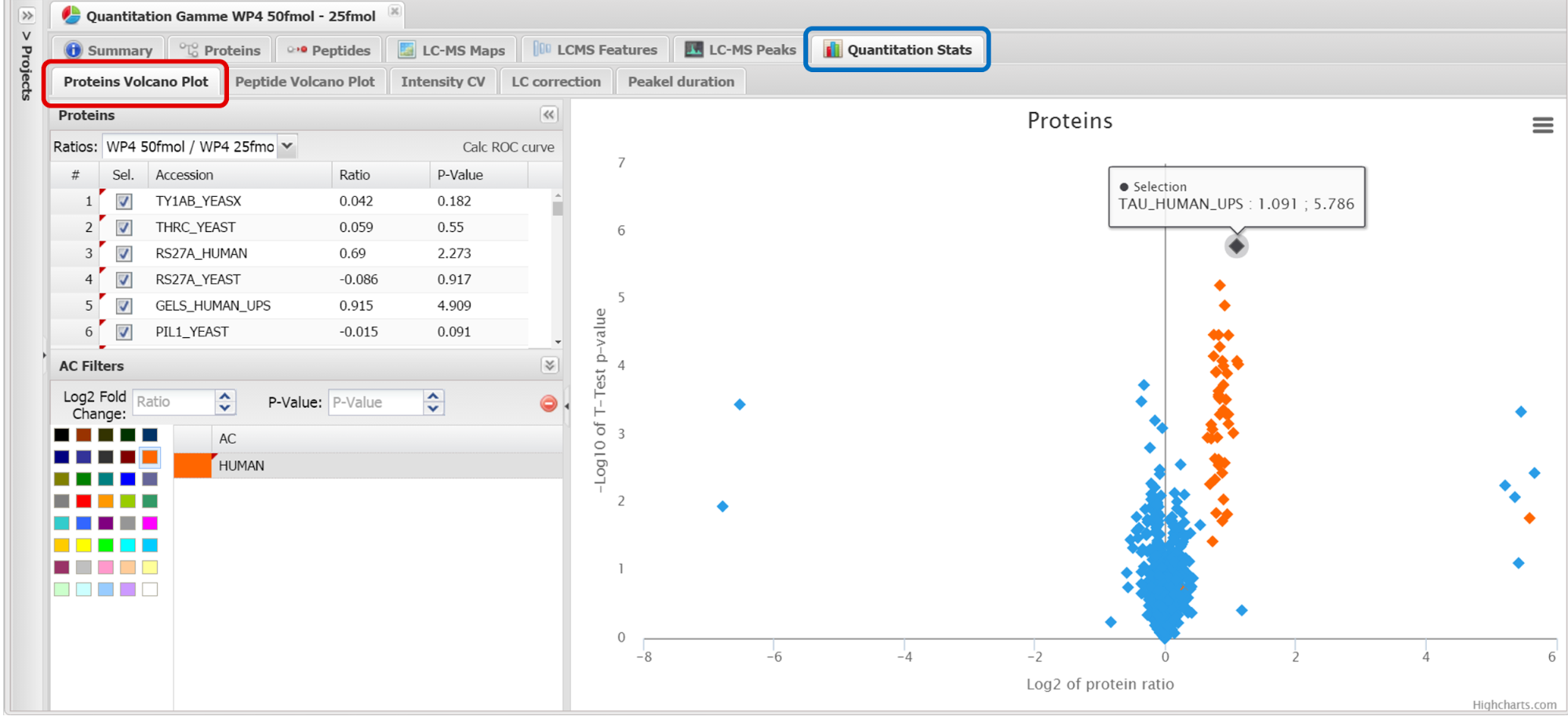
Proline User Guide
Release 2.0
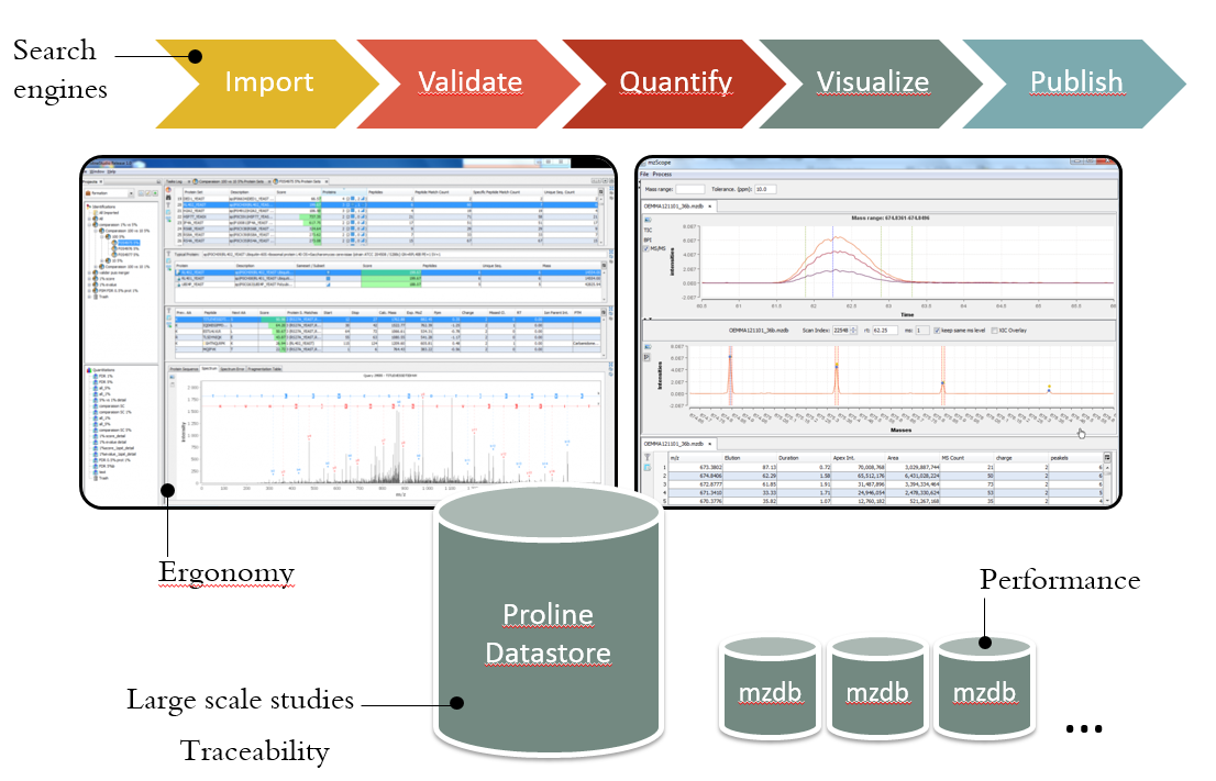
Proline is a suite of software and components dedicated to mass spectrometry proteomics. Proline lets you extract data from raw files, import results from MS/MS identification engines, organize and store your data in a relational database, process and analyse this data to finally visualize and extract knowledge from MS based proteomics results.
The current version support the following features:
The software suite is based on two main components: a server handling processing tasks and based on relational database management system storing the data generated by the software and two different graphical user interfaces, both allowing users to start tasks and visualize the data: Proline Studio which is a rich client interface and Proline Web the web client interface. An additional component called ProlineAdmin dedicated to system administrators to setup and manage Proline.
Read the Concepts & Principles documentation to understand the main concepts and algorithms implemented in Proline.
Find quick answer to your questions in this How to section.
This procedure is detailed in the mzDB Documentation section.
Proline Concepts & Principles
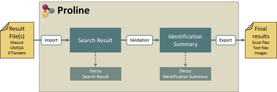
Proline considers different types of identification data: Result Files, Search Results and Identification Summaries which will be defined in the following sections. All these data are connected according to this chart:
A Result File is the file created by a search engine when a search is submitted. OMSSA (.omx files), Mascot (.dat files) and X!Tandem (.xml files) search engines are currently supported by Proline. Generic mzIdentML files could also be imported.
A first version for MaxQuant support has been implemented. It is possible to import only search result or to import search result as well as quantitation (beta version) values from MaxQuant files.
A first step when using Proline is to import Result Files through Proline Studio or Proline Web.
Search engines may provide different types of searches for MS and MS/MS data. It is important to highlight that the Result File content depends on the search type. Proline only supports MS/MS ions searches at this point.
A Search Result is the raw interpretation of a given set of MS/MS spectra given by a search engine or a de novo interpretation process. It contains one or many peptides matching the submitted MS/MS spectra (PSM, i.e. Peptide Spectrum Match), and the protein sequences these peptides belong to. The Search Result also contains additional information such as search parameters, used protein sequence databank, etc.
A Search Result is created when a Result File (Mascot .dat file, OMSSA .omx or a X! Tandem .xml) is imported in Proline. In the case of a target-decoy search, two Search Results are created: one for the target PSMs, one for decoy PSMs.
Importing a Result File creates a new Search Result in the database which contains the following information:
The PSM score corresponds to Mascot ion score.
The PSM score corresponds to the negative common logarithm of the E-value:
Note: Proline only supports OMSSA Result Files generated with the 2.1.9 release.
The X!Tandem standard hyperscore is used as a PSM score.
Note: Proline supports X!Tandem Result Files generated with the Sledgehammer release (or later).
Proline handles decoy searches performed from two different strategies:
Decoy and Target Search Result
See Search Result to view which information is saved.
An Identification Summary is a set of identified proteins inferred from a subset of the PSM contained in the Search Result. The subset of PSM taken into account are the PSM that have been validated using a filtering process (example: PSM fulfilling some specified criteria such as score greater than a threshold value).
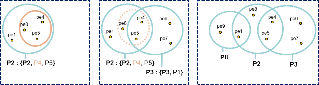
All peptides identifying a protein are grouped in a Peptides Set. A same Peptides Set can identify many proteins, represented by one Proteins Set. In this case, one protein of this Protein Set is chosen to represent the set, it is the Typical Protein. If only a subset of peptides identify a (or some) protein(s), a new Peptide Set is created. This Peptide Set is a subset of the first one, and identified Proteins are Subset Proteins.
All peptides sets and associated protein sets are represented, even if there are no specific peptides. In both cases above, no choice is done on which protein set / peptide set to keep. These protein sets could be filtered after inference (see Protein sets filtering).
There are multiple algorithms that could be used to calculate the Proteins and Protein Sets scores. Proteins scores are computed during the importation phase while Protein Sets scores are computed during the validation phase.
Each individual protein match is scored according to all peptide matches associated with this protein, independently of any validation of these peptide matches. The sum of the peptide matches scores is used as protein score (called standard scoring for Mascot result files).
Each individual protein set is scored according to the validated peptide matches belonging to this protein set (see inference).
The score associated to each identified protein (or protein set) is the sum of the score of all peptide matches identifying this protein (or protein set). In case of duplicate peptide matches (peptide matched by multiple queries) only the match with the best score is considered.
This scoring scheme is also based on the sum of all non-duplicate peptide matches score. However the score for each peptide match is not its absolute value, but the amount that it is above the threshold: the score offset. Therefore, peptide matches with a score below the threshold do not contribute to the protein score. Finally, the average of the thresholds used is added to the score. For each peptide match, the “threshold” is the homology threshold if it exists, otherwise it is the identity threshold. The algorithm below illustrates the MudPIT score computation procedure:
Protein score = 0
For each peptide match {
If there is a homology threshold and ions score > homology threshold {
Protein score += peptide score - homology threshold
} else if ions score > identity threshold {
Protein score += peptide score - identity threshold
}
}
Protein score += 1 * average of all the subtracted thresholds
The benefit of the MudPIT score over the standard score is that it removes many of the junk protein sets, which have a high standard score but no high scoring peptide matches. Indeed, protein sets with a large number of weak peptide matches do not have a good MudPIT score.
This scoring scheme, introduced by Proline, is a modified version of the Mascot MudPIT one. The difference with the latter is that it does not take into account the average of the substracted thresholds. This leads to the following scoring procedure:
Protein score = 0
For each peptide match {
If there is a homology threshold and ions score > homology threshold {
Protein score += peptide score - homology threshold
} else if ions score > identity threshold {
Protein score += peptide score - identity threshold
}
}
This score has the same benefits than the MudPIT one. The main difference is that the minimum value of this modified version will be always close to zero while the genuine MudPIT score defines a minimum value which is not constant between the datasets and the proteins (i.e. the average of all the subtracted thresholds).
There are several ways to calculate FDR depending on the database search type. In Proline the FDR is calculated at peptide and protein levels using the following rules:

Note: when computing PSM FDR, peptide sequences matching a Target Protein and a Decoy Protein is taken into account in both cases.

Once a result file has been imported and a search result created, the validation is performed in four main steps:
Finally, the Identification Summary issued from these steps is stored in the identification database. Different validation of a Search Result can be performed and a new Identification Summary of this Search Result is created for each validation.
When validating a merged Search Result, it is possible to propagate the same validation parameters to all childs Search Results. In this case Peptide Matches filtering and Validation will be applied on childs as well as Protein Sets filtering. Note: actually, Protein Sets validation is not propagated to childs Search Results.
Peptide Matches identified in search result can be filtered using one or multiple predefined filters (described hereafter). Only validated peptide matches will be considered for further steps.
All PSMs which score is lower than a given threshold are invalidated.
This filtering is performed after having temporarily joined target and decoy PSMs corresponding to the same query (only really needed for separated forward/reverse database searches). Then for each query, PSMs from target and decoy are sorted by score. A rank (Mascot pretty rank) is computed for each PSM depending on their score position: PSM with almost equal score (difference < 0.1) are assigned the same rank. All PSMs with rank greater than specified one are invalidated.
PSMs corresponding to short peptide sequences (length lower than the provided one) can be invalidated using this parameter.
Allows to filter PSMs by using the Mascot expectation value (e-value) which reflects the difference between the PSM score and the Mascot identity threshold (p=0.05). PSMs having an e-value greater than the specified one are invalidated.
Proline is able to compute an adjusted e-value. It first selects the lowest threshold between the identity and homology ones (p=0.05). Then it computes the e-value using this selected threshold. PSMs having an adjusted e-value greater than the specified one are invalidated.
Given a specific p-value, the Mascot identity threshold is calculated for each query and all peptide matches associated to the query with a score lower than calculated identity threshold are invalidated.
When parsing Mascot result file, the number of PSM candidate for a spectra is saved and could be used to recalculate identity threshold for any p-value.
Given a specific p-value, the Mascot homology threshold is inferred for each query and all peptide matches associated to the query with a score lower than calculated homology threshold are invalidated.
This filter validates only one PSM per Query. To select a PSM, following rules are applied:
For each query:
For testing purpose, it is possible to request for this filter to be executed after Peptide Matches Validation (see below). In this case, the requested FDR in validation step is modified by this filter. This is just to confirm the need or not of this filter and to validate the way we apply it!
This filter validates only one PSM per Pretty Rank. If you choose this filter + a pretty rank filter you should have the same behaviour than the “Single PSM per Query Filter”.
In order to choose the PSM, following rules are applied:
For Pretty Rank of each query:
For testing purpose, it is possible to request for this filter to be executed after Peptide Matches Validation (see below). In this case, the requested FDR in validation step is modified by this filter. This is just to confirm the need or not of this filter and to validate the way we apply it!
Specify an expected FDR and tune a specified filter in order to obtain this FDR. See how FDR is calculated.
Once previously described prefilters have been applied, a validation algorithm can be run to control the FDR: given a criteria, the system estimates the better threshold value in order to reach a specific FDR.
Filtering applied during validation is the same as Protein Sets Filtering
Once prefilters (see above) have been applied, a validation algorithm can be run to control the FDR. See how FDR is calculated.
At the moment, it is only possible to control the FDR by changing the Protein Set Score threshold. Three different protein set scoring functions are available.
Given an expected FDR, the system tries to estimate the best score threshold to reach this FDR. Two validation rules (R1 and R2) corresponding to two different groups of protein sets (see below the detailed procedure) are optimized by the algorithm. Each rule defines the optimum score threshold allowing to obtain the closest FDR to the expected one for the corresponding group of protein sets.
Here is the procedure used for FDR optimization:
The separation of proteins sets in two groups allows to increase the power of discrimination between target and decoy hits. Indeed, the score threshold of the G1 group is often much higher than the G2 one. If we were using a single average threshold, this would reduce the number of G2 validated proteins, leading to a decrease in sensitivity for a same value of FDR.
Any Identification Summary, generated by validation or merging could be filtered.
Filtering consists in invalidating Protein Sets which doesn't follow specified criteria. Invalidated Protein Sets are not been taken into account for further algorithms or display.
Available filtering criteria are defined below.
This filter invalidates protein sets that don't have at least x peptides identifying only that protein set. The specificity is considered at the DataSet level.
This filtering go through all Protein Sets from worse score to best score. For each, if the protein set is invalidated, associated peptides properties are updated before going to next protein set. Peptide property is the number of identified protein sets.
This filter invalidates protein sets that don't have at least x peptides identifying that protein set, independently of the number of protein sets identified by the same peptide.
This filtering go through all Protein Sets. For each, if the protein set is invalidated, associated peptides properties are updated before going to next protein set. Peptide property is the number of identified protein sets.
This filter invalidates protein sets that don't have at least x different peptide sequences (independently of PTMs) identifying that protein set.
This filtering go through all Protein Sets from worse score to best score. For each, if the protein set is invalidated, associated peptides properties are updated before going to next protein set. Peptide property is the number of identified protein sets.
This filter invalidates protein sets which score is below the a given value.
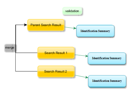
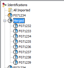
Two king of merge is allowed in Proline.
Merging several Search Results consists in creating a parent Search Result which contains the best child PSM for each peptide. The best PSM is the PSM with the highest score.
Merging several Search Results consists in creating a parent Search Result which contains all child PSMs from each child Search Result. Warning: Depending on the size of the child Search Result, this operation may be long and size of project databases may increase quickly.
Once Search Results have been merged, only Parent Search Result can be directly validated. However, this validation could be propagated to the child. In this case Peptide Matches filtering and Validation will be applied on childs as well as Protein Sets filtering. Note: actually, Protein Sets validation is not propagated to childs Search Results.
Another merge algorithm could be used: see Merge Identification Summaries
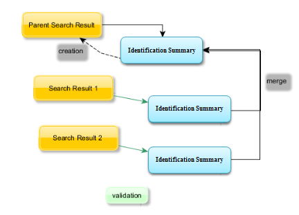
Merging several Identification Summaries consists in creating a parent Identification Summary which contains the best child PSM for each peptide ( The best PSM is the PSM with the highest score).
A Search Result corresponding to this parent Identification Summary is generated and Protein Inference is applied.
Merging several Identification Summaries consists in creating a parent Identification Summary which contains all validated PSMs from child Identification Summaries.
A Search Result corresponding to this parent Identification Summary is generated and Protein Inference is applied.
Even in union mode this operation should less time and size consuming as only validated PSMs are taken into account.
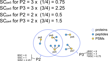
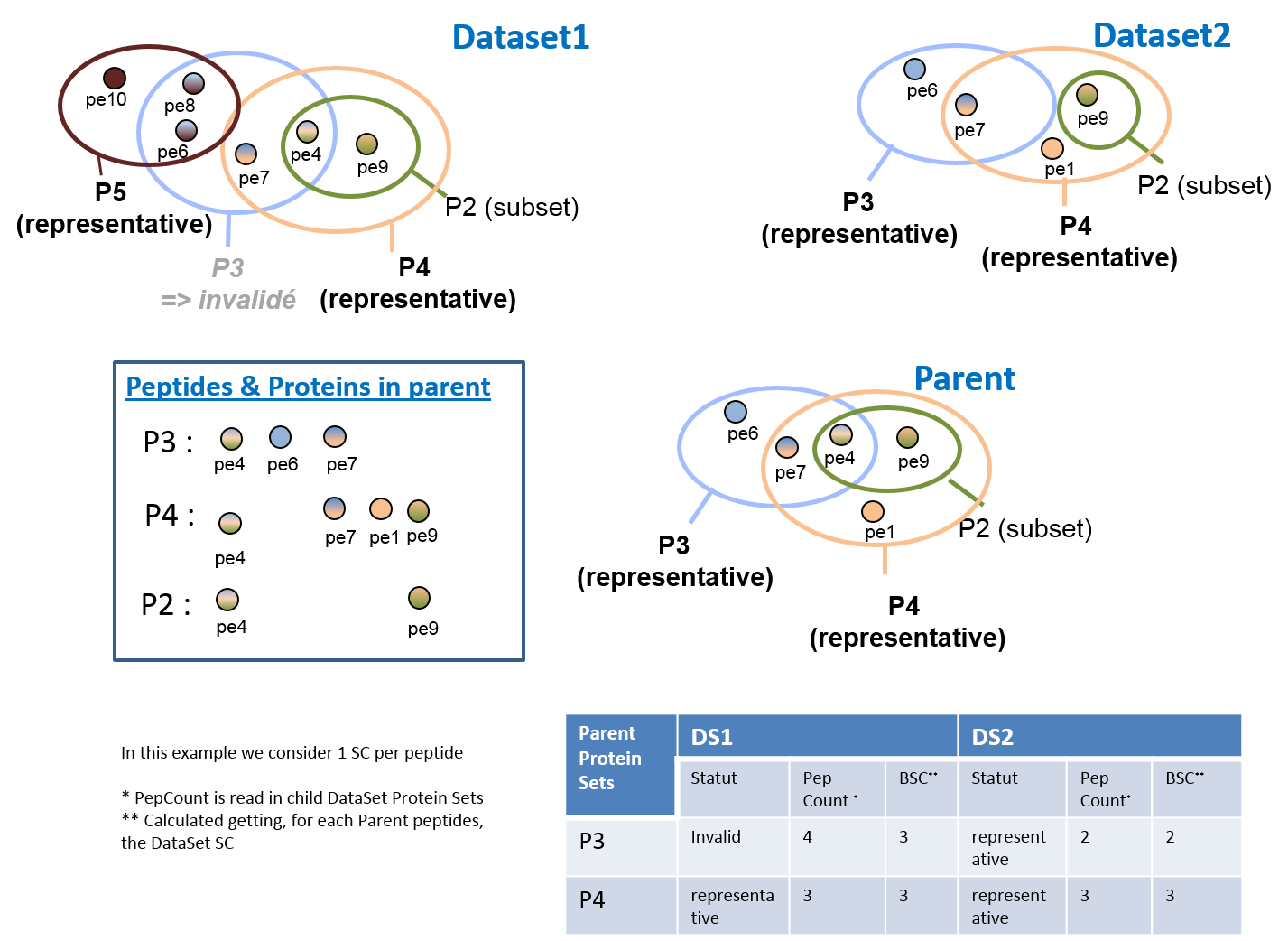
Example calculation of spectral count
The peptide specificity and the spectral count weight could be defined in the context of the Identification Summary where the spectral count is calculated as shown in previous schema. It could also could be done using another Identification Summary as reference, like using the common parent Identification Summary. This allow to consider only identified and validated protein in the merge context.
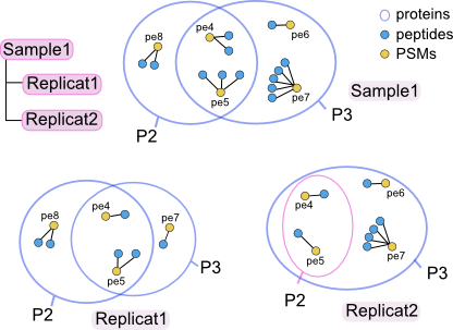
If we consider the following case, where Sample1 Identification Summary is the merge of Replicat1 and Replicat2.
If the spectral count calculation is done at each child level, aligning protein sets identified in parent to protein sets in child, we get the following result:
Sample1 Protein Sets | Replicat1 | Replicat2 | ||||||
Ref Prot. | BSC | SSC | WSC | Ref Prot. | BSC | SSC | WSC | |
P2 | P2 | 5 | 2 | 4 | P3 | 7 | 7 | 7 |
P3 | P3 | 4 | 1 | 2 | P3 | 7 | 7 | 7 |
We can see that when different parent protein sets are seen as one protein set in a child, the spectral count is biased. This calculation was not retain!
Now, if we align on child protein rather than protein sets, we get the following result:
Sample1 Protein Sets | Replicat1 | Replicat2 | ||||||
Ref Prot. | BSC | SSC | WSC | Ref Prot. | BSC | SSC | WSC | |
P2 | P2 | 5 | 2 | 4 | P2 | 2 | 0 | 0 |
P3 | P3 | 4 | 1 | 2 | P3 | 7 | 7 | 7 |
Again, when considering specificity at child level, the result of spectral count in Replicat2 is not representative, as it has a null SSC and WSC. This calculation was not retain!
A way to make some correction is to define the specificity of the peptide and their weight at the parent level, and apply it at the child level. Therefore, specific peptides for P2 is pe8 and for P3 it is pe6 and pe7. For peptide weight, if we consider pe4 for example, it will be define as follow:
The spectral count result will thus be:
Sample1 Protein Sets | Replicat1 | Replicat2 | ||||||
Ref Prot. | BSC | SSC | WSC | Ref Prot. | BSC | SSC | WSC | |
P2 | P2 | 5 | 2 | 2.75 | P2 | 2 | 0 | 0.5 |
P3 | P3 | 4 | 1 | 3.25 | P3 | 7 | 5 | 6.5 |
NOTE:
In case of multiple level hierarchy (Sample → Condition1 vs Condition2 → 3 replicates by conditions), it could make sense to calculate the spectral count weight at “Condition1” and “Condition2” levels rather than “Sample” level to keep the difference involved by the experiment condition.
Actually, spectral count is calculated for a set of hierarchy related Identification Summaries. In other words, this means that Identification Summaries should have a common parent. The list of protein to compare or to consider is created at the parent level as the peptide specificity. User can select the dataset where the shared peptides spectral count weight is calculated. (See previous chapter)
Firstly, the peptide spectral count is calculated using following rules
Once, peptide spectral count is known for each peptide, protein spectral count is calculated using following rules
When running SC even on a simple hierarchy (1 parent, 2 childs) in some case we obtain a BSC less than peptide count. This occurs only for Invalid Protein Sets. Invalid Protein Sets are the one that are present at the parent level but was filtered at child level (filter on specific peptide for example).
Indeed, the peptide count value is read in the child Protein Sets. On the other hand, the BSC is calculated by getting the spectral count information at child level for each peptide identified at parent level. If a Protein Set is invalidated, its peptide are not taken into account while merging so some of them could be missing at parent level if there were not identified in the other child.
This case is illustrated here
This section will describes in details the quantitation principles and concepts implemented in Proline:
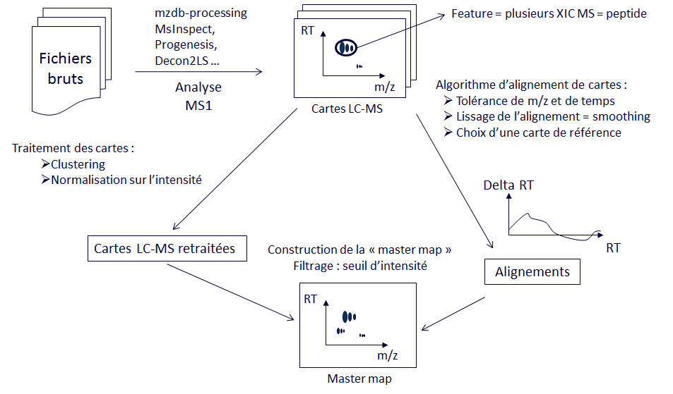
Analyzing Label-free LC-MS data requires a series of algorithms presented below.
Figure 1 : overview of the different stages of label-free LC-MS data processing |
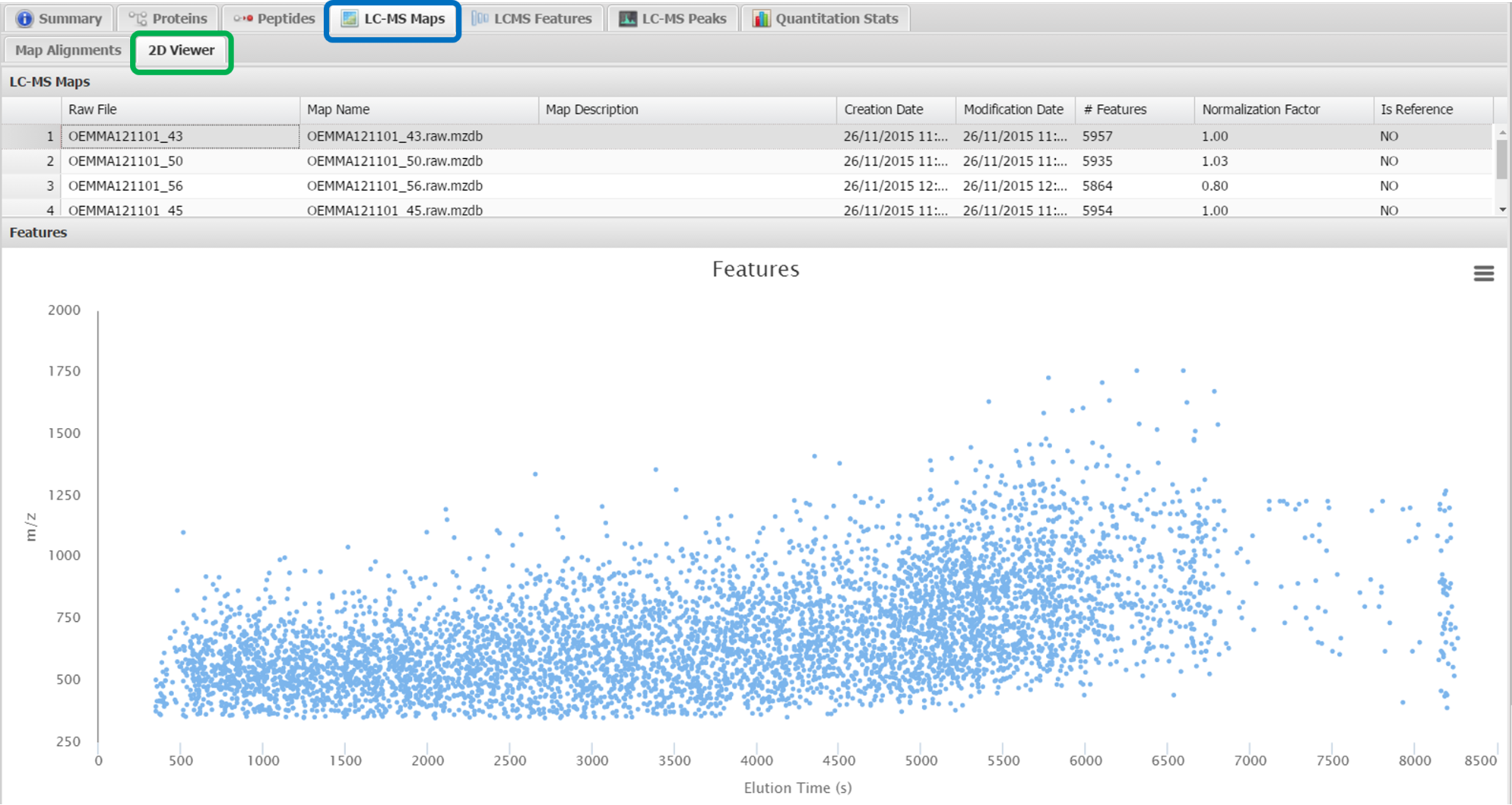
LC-MS maps are created directly through Proline by using its own algorithms.
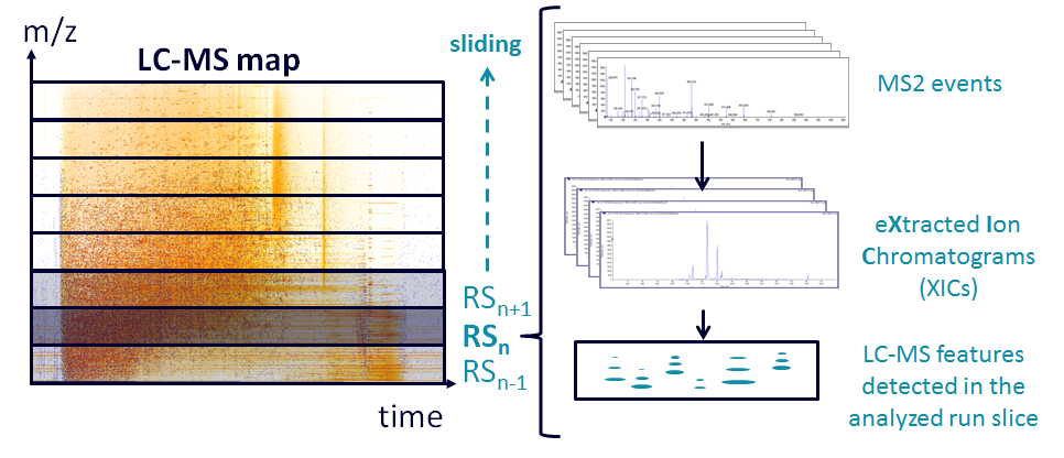
These algorithms take advantage of the mzDB file format to process ions not scan by scan but in the m/z dimension by processing elution peaks in LC-MS regions of 5 Da width, also called run slices.
Proline provides multiple algorithms
The preferred algorithm is Proline is the one performing an unsupervised detection of chromatographic peaks (also called peakels).
The detection of all the MS signals is made in a single iteration on all the run slices of the mzDB file. Thus all peptide signals whose mass is contained in a specific run slice are detected simultaneously.
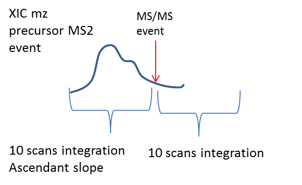
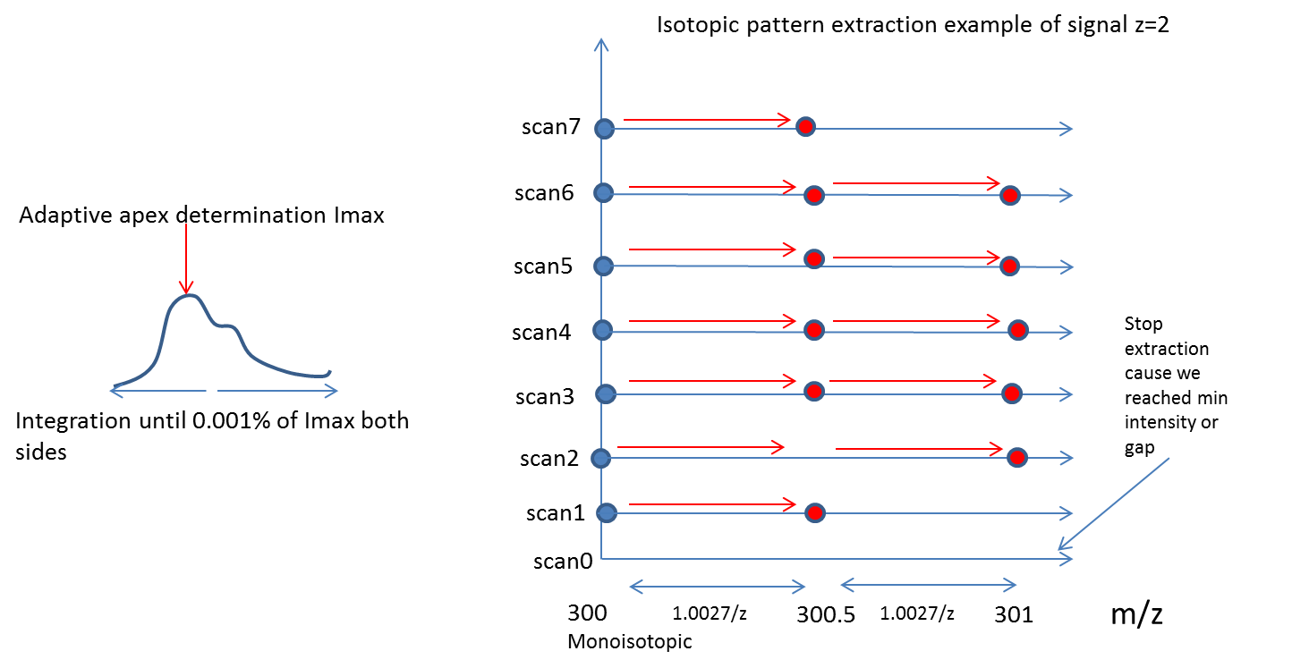
In a given run slice, m/z peaks are first sorted in descending intensity order. Starting from the most intense m/z peak, the algorithm searches for the peak of the same m/z value in the preceding and following MS1 scans according to a user-defined m/z tolerance depending on the mass analyzer. The lookup procedure stops as soon as the m/z peak is absent in more than a predefined number of consecutive scans. Once collected this m/z peak list, which is comparable to a chromatogram, is then smoothed using a Savitzky-Golay filter and split in the time dimension to form elution peaks by applying a peak picking procedure that searches for significant minima and maxima of signal intensity. At this stage, the process returns a list of elution peaks defined by an m/z value, an apex elution time and an elution time range.
The deisotoping of the obtained peaks is performed separately using two possible algorithms:
This alternative algorithm performs a target signal extraction rather than an unspervised detection. It has been now deprecated but I think it is important to understand the differences with the unsupervised approach.
In this second algorithm, we consider each MS/MS event triggered by the spectrometer as an evidence for the presence of a peptide ion. Each of these events provides a set of information about the targeted precursor ion: the m/z ratio (assuming it is monoisotopic), the moment when the MS/MS has been triggered (usually not the maximum of the elution peak) and the charge state of the ion. The first and second information can be considered as close coordinates for the peptide signal on the LC-MS map. The charge state (z) can provide additional information to simplify the extraction of different isotopes of the features which are approximately separated by 1/z. For each MS/MS event:
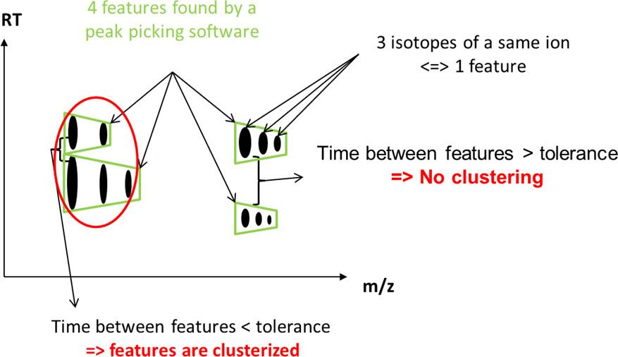
Maps generated with peak picking algorithms cannot be 100% reliable and often contain redundant signals, corresponding to the same compound. Furthermore, modified peptides having the same sequence can have different PTM polymorphisms that can give different MS signals with the same m/z ratio but having slightly different retention times. Comparing LC-MS maps with such cases is a problem as it may lead to an inversion of feature matches between maps. Creating feature clusters is a way to avoid this issue. This operation is called “Clustering” (cf. figure 2).
Figure 2: grouping features into cluster. All features with the same charge state, close m/z ratio and retention times are grouped in a single cluster. The other features are stored without clustering. |
Feature clustering consists in grouping, in a given LC-MS map, the features with the same charge state, close in retention time and m/z ratio (default tolerances are respectively 15 seconds and 10 ppm). Some metrics are calculated for each cluster (equivalent to those used for the features):
The resulting maps are “cleaner”, thus reducing ambiguities for map alignment and comparison. Quantitative data extracted from these maps will be processes in the following steps. It is necessary to eliminate the ambiguities found by the clustering step. To do so, it is possible to rely on the information given by the search engine on each identified peptide. If some ambiguities remain, the end user must be aware of them and be able to either manually handle them or either exclude them from the analysis.
Note: do not mix up clustering and deconvolution which consists in grouping all the charge states detected for a single molecule.
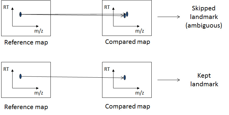
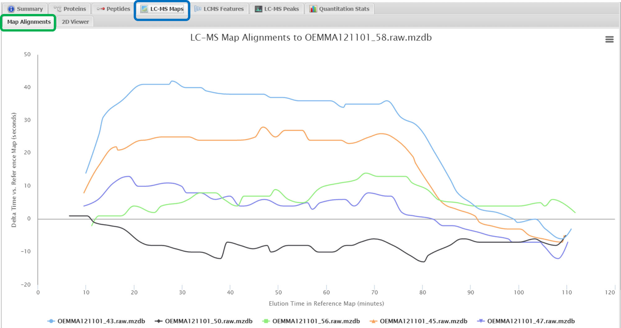
Because chromatographic separation is not completely reproducible, LC-MS maps must be aligned before being compared. The first step of the alignment algorithm is to randomly pick a reference map and then compare every other map to it. On each comparison, the algorithm will determine all possible matches between detected features, considering time and mass windows (the default values are respectively 600 seconds and 10 ppm). Only landmarks involving unambiguous links between the maps (only one feature on each map) are kept (cf. figure 3).
Figure 3 : Matching features with the reference map respecting a mass (10 ppm) and time tolerance (600 s) | |
The result of this alignment algorithm can be represented with a scatter plot (cf. figure 5).
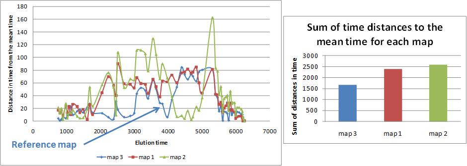
The algorithm completes this alignment process several times with randomly chosen reference maps. Then it sums the absolute values of the distance between each map to an average map (cf. figure 4). The map with the lowest sum is the closest to the other maps and will be considered as the final reference map from this point.
Figure 4: Selection of the reference map. The chart on the left shows the time distances between each map and the average map obtained by multiple alignments. The chart on the right summarizes the integration of each curve in the chart on the left. The map closest to the average map is selected as the reference map. |
Two algorithms have been implemented to make this selection.
This algorithm considers every possible couple between maps:
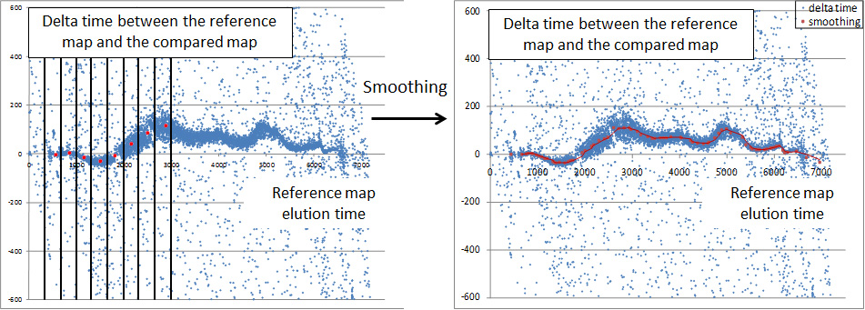
The last thing to do is to find the path going through the regions with the highest density of points in the scatter plot. This step was implemented using a moving median smoothing (cf. figure 5).
Figure 5: Alignment smoothing of two maps using a moving median calculation. The scatter plot represents the time variation (in seconds) of multiple landmarks (between the compared map and the reference map) against the observed time (in seconds) in the reference map. A user-defined window is moved along the plot, computing on each step a median time difference (left plot). The smoothed alignment curve is constituted of all the median values (right plot). |
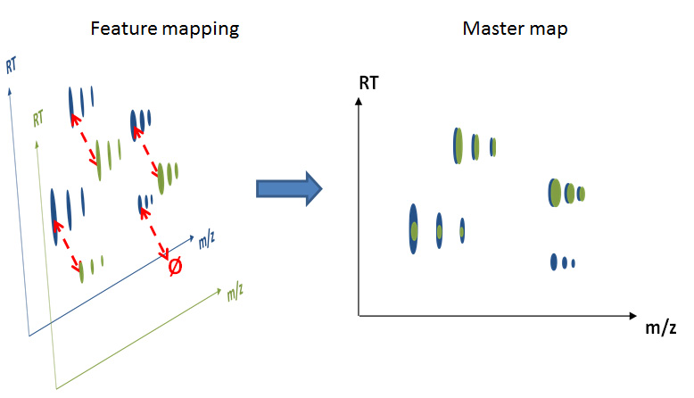
Once the maps have been corrected and aligned, the final step consists in creating a consensus map or master map. It is produced by searching the best match for each feature detected on different maps. The master map can be seen as a representation of all the features detected on the maps, without redundancy. (cf. figure 6).
Figure 6: Creation of the master map by matching the features detected on two LC-MS maps. The elution times used here are the ones corrected by the alignment step. The intensity of a feature can vary from one map to another, it can also happen that a feature appears in only one map. |
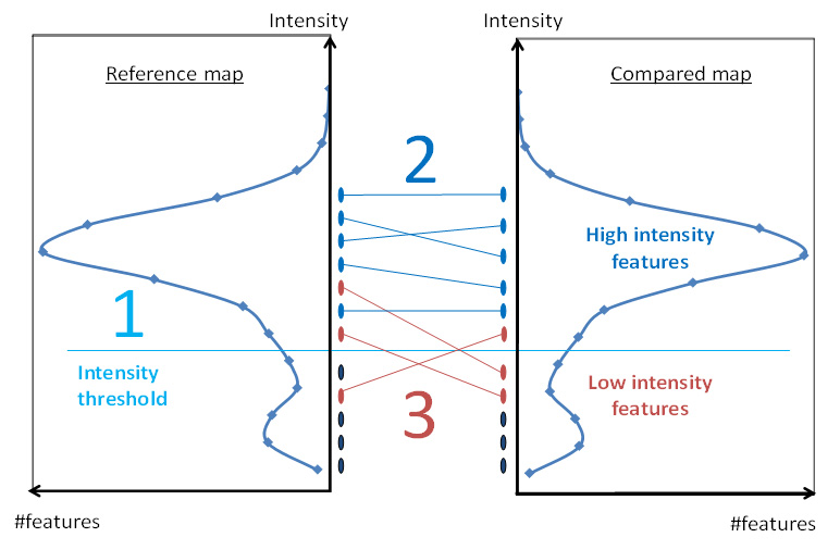
During the creation of the master map, the algorithm first considers matches for the most intense features (higher than a given threshold), and then consider the other features only if they match a feature with a high intensity in another map. This is done in order to avoid to include background noise to the master map (cf. figure 7).
Figure 7: Distribution of the intensities of the maps considered to build the master map. The construction is done in 3 steps: 1) removing features with a normalized intensity lower than a given threshold 2) matching the most intense features 3) features without matches in at least one map are compared again with the low intensity features, put aside in first step. “Predicted time extractor” algorithmThis algorithm is used for cross-assignment, when a peptidic signal is detected in a file but does not have an equivalent signal in another one (frequently in DDA). In this case, the algorithm tries to extract some signal from the file where the signal has not been found. The aim of this algorithm is to reduce the number of missing values.
|
It has been seen that ambiguous features with close m/z and retention times can be grouped into clusters. Other conflicts are also generated during the creation of the master map due to wrong matches. Adding the peptide sequence is the key to solve these conflicts by identifying without ambiguity a feature. Proline has access to the list of all identified and validated PSMs as well as the identifier (id) of each MS/MS spectrum related to an identification. This means that the link between the scan id and the peptide id is known. On the other hand the list of MS/MS events simultaneous to the elution window of each feature is known. For each of these events the corresponding peptide sequences can be retrieved. If only one peptide sequence is found for the master feature, it is be kept as it is. Otherwise the master feature is cloned in order to have one feature per peptide sequence. During this duplication step the daughter features are distributed on the new master features according to the identified peptide sequences.
When the master map is created some intensity values could be missing. Proline reads the mzDB files to reduce the number of missing values, using the expected coordinates (m/z – RT) for each missing feature to extract new features. These new extractions are added to copies of the daughters and the master maps. This gives a new master map with a limited number of missing values.
The comparison of LC-MS maps is confronted to another problem which is the variability of the MS signals measured by the instrument. This variability can be technical or biological. Technical variations between MS signals in two analyses can depend on the injected quantity of material, the reproducibility of the instrument configuration and also the software used for the signal processing. The observed systematic biases on the intensity measurements between two successive and similar analysis are mainly due to errors in the total amount of injected material in each case, or the LC-MS system instabilities that can cause variable performances during a series of analysis and thus a different response in MS signal for peptides having the same abundance. Data may not be used if the difference is too important. It is always recommended to do a quality control of the acquisition before considering any computational analysis. However, there are always biases in any analytic measurement but they can usually be fixed by normalizing the signals. Numerous normalization methods have been developed, each of them using a different mathematical approach (Christin, Bischoff et al. 2011). Methods are usually split in two categories, linear and non-linear calculation methods, and it has been demonstrated that linear methods can fix most of the biases (Callister, Barry et al. 2006). Three different linear methods have been implemented in Proline by calculating normalization factors as the ratio of the sum of the intensities, as the ratio of the median of the intensities, or as the ratio of the median of the intensities.
How to calculate this factor:
How to calculate this factor:
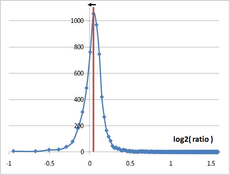
This last strategy has been published in 2006 (Dieterle, Ross et al. 2006) and gives the best results. It consists in calculating the intensity ratios between two maps to be compared then set the normalization factor as the inverse value of the median of these ratios (cf. figure 8). The procedure is the following:
Figure 8 : Distribution of the ratios transformed in log2 and calculated with the intensities of features observed in two LC-MS maps. The red line representing the median is slightly off-centered. The normalization factor is equal to the inverse of this median value. The normalization process will refocus the ratio distribution on 0 which is represented by the black arrow. |
Proline makes this normalization process for each match with the reference map and has a normalization factor for each map, independently of the choice of the algorithm. The normalization factor for the reference map is equal to 1.
Once the master map is normalized, it is stored in the Proline LCMS database and used to create a “QuantResultSummary”. This object links the quantitative data to the identification summaries validated in Proline. This “QuantResultSummary” is then stored in the Proline MSI database (cf. figure 9).
Figure 9: From raw files to the « QuantResultSummary » object. |
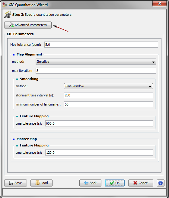
The first quantitation step as well as the advanced quantitation (see Quantitation: principles) has some parameters that could be modified by the user.
Here is the description of the parameters that could be modified by the user.
These parameters are used by signal extraction algorithms .
Clustering must be applied to the imported LC-MS maps to group features that are close in time and m/z. This step reduces ambiguities and errors that could occur during the feature mapping phase.
This is an important step in the LCMS process. It consists in aligning maps of the map set to correct the RT values. RT shifts of shared features between the compared maps follow a curve reflecting the fluctuations of the LC separation. The time deviation trend is obtained by computing a moving median using a smoothing algorithm. This trend is then used as a model of the alignment of the compared LC-MS maps. This model provides a basis for the correction of RT values.
Then all other maps are aligned to this computed reference map and their retention times are corrected.
When alignment is done, a trend can be extracted with a smoothing method permitting the correction of the aligned map retention time.
This step consists in creating the “master map” (also called consensus map), this map resulting from the superimposition of all compared maps.
If you choose Relative intensity for master feature filter type, the only possibility you have is percent, so features which intensities are beyond the relative intensity threshold in percentage of the median intensity are removed. If you choose Intensity for master feature filter type, you also have only one possibility at the moment of the intensity method: basic. Features which intensities are beyond the intensity threshold are removed and not considered for the master map building process.
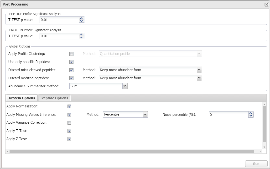
This procedure is used to compute ratios of peptide and protein abundances. Several filters can also be set to increase the quality of quantitative results.
Here is the description of the parameters that could be modified by the user.
Peptide abundances can be summarized into protein abundances using several mathematical methods:
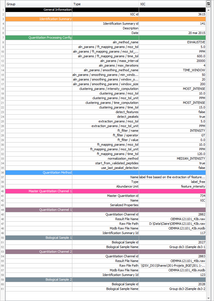
When exporting a whole Identification Summary in an excel file, the following sheets may be generated:
Note: Read the Concepts & Principles documentation to understand main concepts and algorithms used in Proline.
Proline Studio
Calc. Mass: Calculated Mass
Delta MoZ: Delta Mass to Charge Ratio
Exp. MoZ: Experimental Mass to Charge Ratio
Ion Parent Int.: Ion Parent Intensity
Missed Cl.: Missed Cleavage
Modification D. Mass: Modification Delta Mass
Modification Loc.: Modification Location
Next AA: Next Amino-Acid
Prev. AA: Previous Amino-Acid
Protein Loc.: Protein Location of the Modification
Protein S. Matches: Protein Set Matches
PSM: Peptide Spectrum Match
PTM: Post Translational Modification
PTM D. Mass: PTM Delta Mass
RT: Retention Time
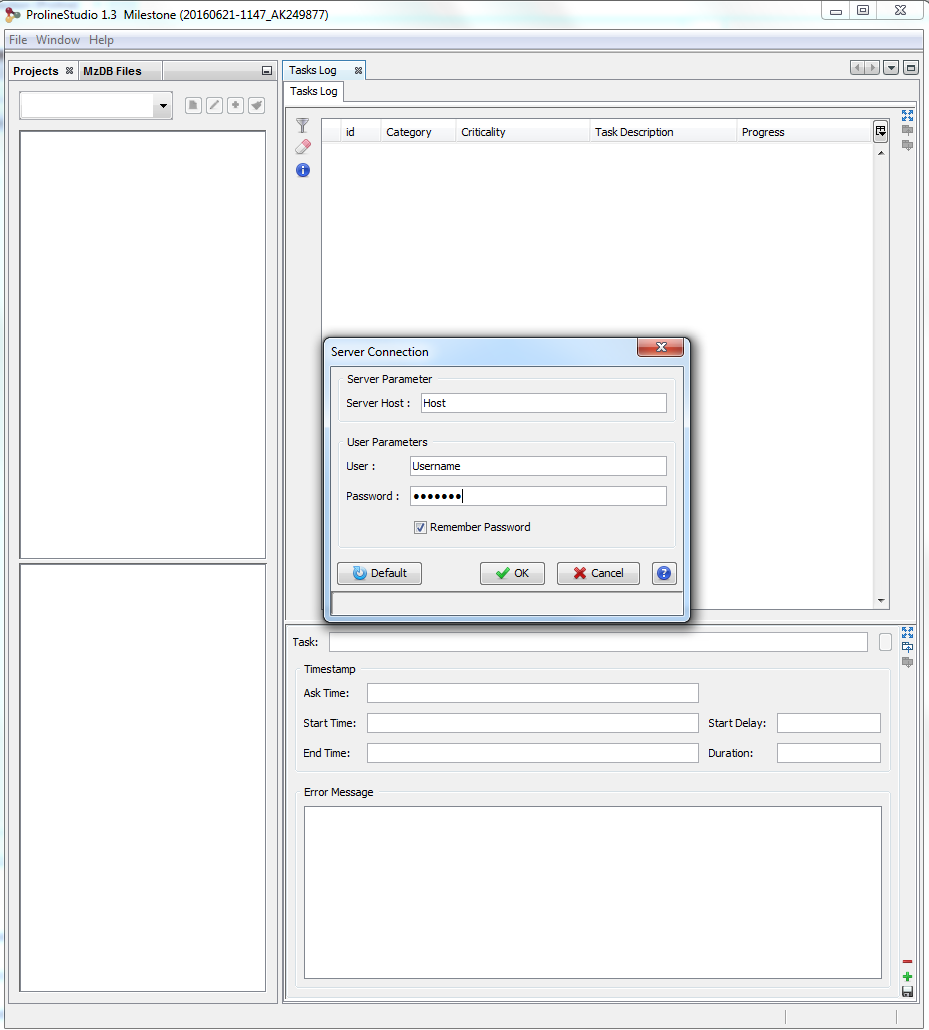
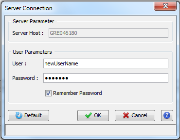
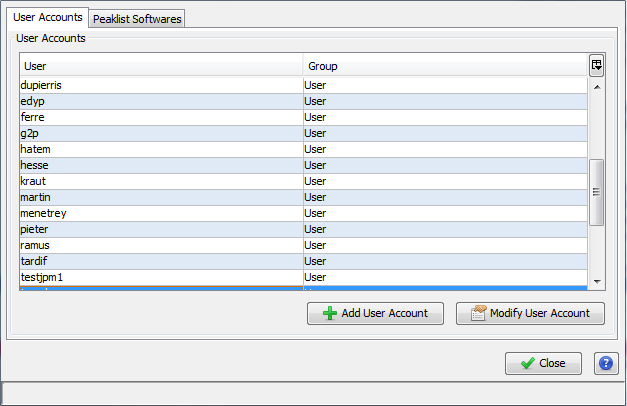
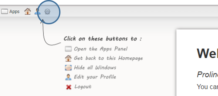
When you start Proline Studio for the first time, the Server Connection Dialog is automatically displayed.
You must fill the following fields:
- Server Host: this information must be asked to your IT Administrator. It corresponds to the Proline server name
- User: your username (an account must have been previously created by the IT Administrator).
- Password: password corresponding to your account (username).
If the field “Remember Password” is checked, the password is saved for future use. Server connection dialog continues to open with Proline Studio, the user though does not need to fill in his password, unless the last one is changed after his last login.
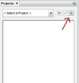
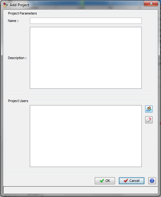
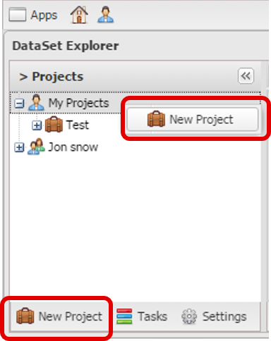
To create a Project, click on “+“ button at the right of the Project Combobox. The Add Project Dialog opens.
Fill the following fields:
- Name: name of your project
- Description: description of your project
You can specify other people to share this new project with them. Then click on OK Button
Creation of a Project can takes a few seconds. During its creation, the Project is displayed grayed with a small hourglass over it.
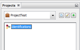
In the Identification tree, you can create a Dataset to group your data
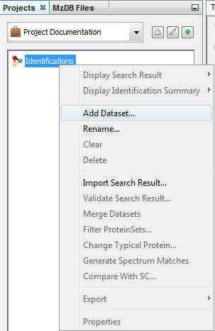
To create a Dataset:
- right click on Identifications or on a Dataset to display the popup.
- click on the menu “Add Dataset…”
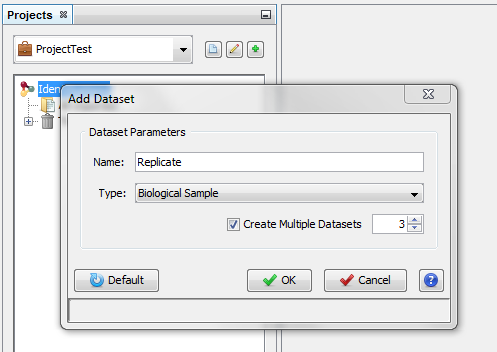
On the dialog opened:
- fill the name of the Dataset
- choose the type of the Dataset
- optional: click on “Create Multiple Datasets” and select the number of datasets you want to create
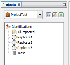
Let's see the result of the creation of 3 datasets named “Replicate”:
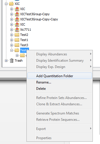
In both Identification and Quantitation tree, you can create Folders to organize your data
To create a Folder :
- right click on Identifications, Quantitations or on a Folder to display the popup.
- click on the menu “Add Identification Folder…” or “Add Quantitation Folder…”
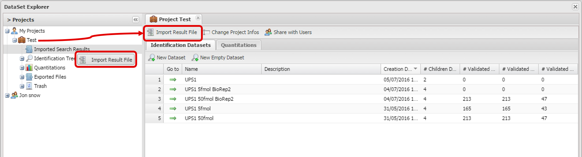
There are two possibilities to import Search Results:
- import multiple Search Results in “All Imported” and put them later in different datasets.
- import directly a Search Result in a dataset.
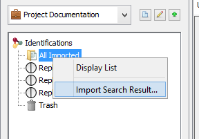
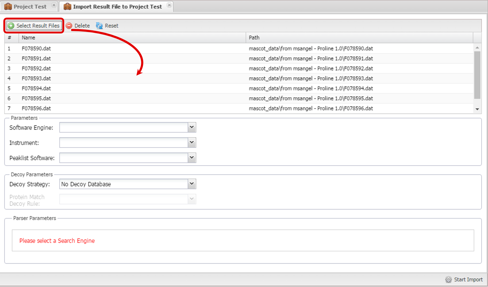
To import in “All Imported”:
- right click on “All Imported” to show the popup
- click on the menu “Import Search Result…”
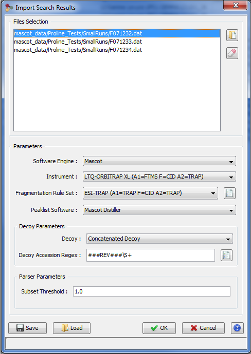
In the Import Search Results Dialog:
- select the file(s) you want to import thanks to the file button (the Parser will be automatically selected according to the type of file selected)
- select the different parameters (see description below)
- click on OK button
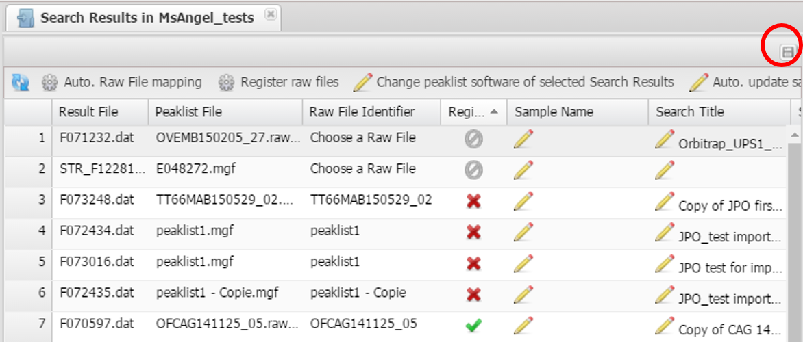
Note 1: You can only browse the files accessible from the server according to the configuration done by your IT Administrator. Ask him if your files are not reachable. (Look for Setting up Mount-points paragraph in Installation & Setup page).
Note 2: Proline is able to import OMSSA files compressed with BZip2.
Note 3: MaxQuant import will generate a dataset hierarchy with the result from the different acquisition.
Parameters description:
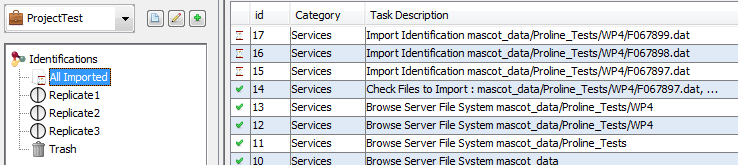
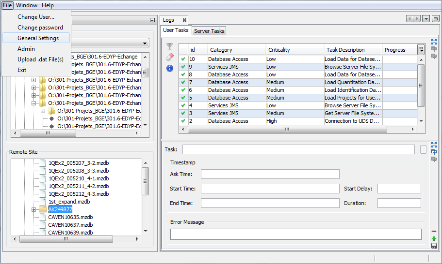
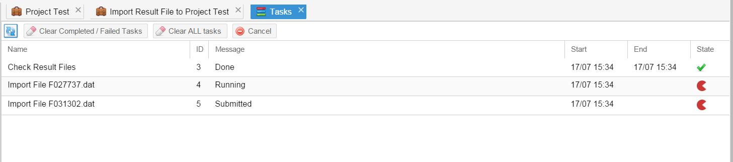
Importing a Search Result can take some time. While the import is not finished, the “All Imported” is shown grayed with an hourglass and you can follow the imports in the Tasks Log Window (Menu Window > Tasks Log to show it).
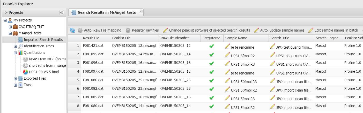
To show all the Search Results imported, double click on “All Imported”, or right click to popup the contextual menu and select “Display List”
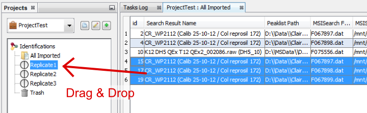
From the All Imported window, you can drag and drop one or multiple Search Result to an existing dataset.
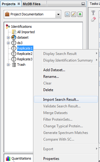
It is possible to import a Search Result directly in a Dataset. In this case, the Search Result is available in “All Imported” too.
To import a Search Result in a Dataset, right click on a dataset and then click on “Import Search Result…” menu. Same dialog and parameters as in “Import in “All Imported”” above will be displayed. |
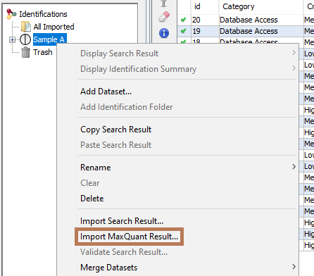
To import a MaxQuant Search Result, right click on a dataset and then select “Import MaxQuant”
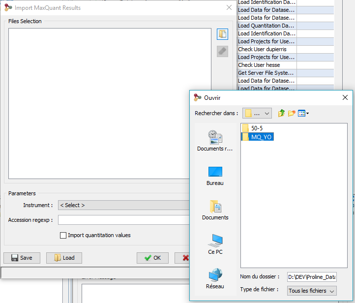
The following dialog will be displayed
- select the directory containing the files generated by MaxQuant. This folder should look like:
<root_folder>\mqpar.xml
<root_folder>\combined\txt\summary.txt
<root_folder>\combined\txt\proteinGroups.txt
<root_folder>\combined\txt\parameters.txt
<root_folder>\combined\txt\msmsScans.txt
<root_folder>\combined\txt\msms.txt
- select the Instrument: mass-spectrometer used for sample analysis different parameters
- specify, if needed, the regular expression to extract protein accessions from MaxQuant protein ids.
- you can choose to import also quantitation data
- click on OK button
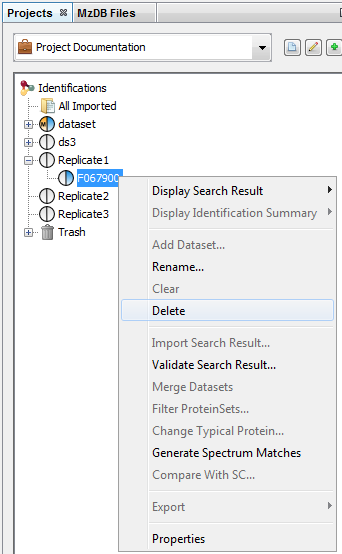
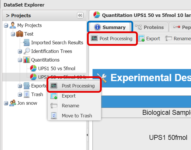
You can delete Search Results, Identification Summaries and Datasets in the data tree. You can also delete XIC or Spectral Counts in the quantitation tree.
Delete the Datasets (identification or quantitation…) from the tree view (Search Result always accessible from “All Imported” view…).
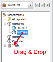
There are two ways to delete data: use the contextual popup or drag and drop data to the Trash.
Select the data you want to delete, right-click to open the contextual menu and click on delete menu.
The selected data is put in the Trash. So it is possible to restore it while the Trash has not been emptied.
Select the data you want to delete and drag it to the Trash. It is possible to restore data while the Trash has not been emptied
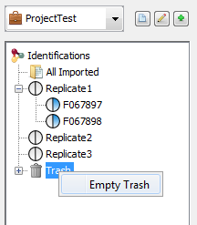
To empty the Trash, you have to Right click on it and select the “Empty Trash” menu.
A confirmation dialog is displayed and if accepted Dataset will be removed from the Trash.
Search Results are not completely removed, you can retrieve them from the “All Imported” window.
It is not possible to delete a Project by yourself. If you need to do it, ask to your IT Administrator.
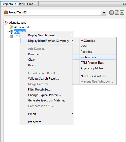
Once user is connected (see Server Connection), it is possible to:
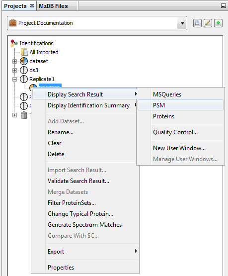
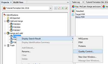
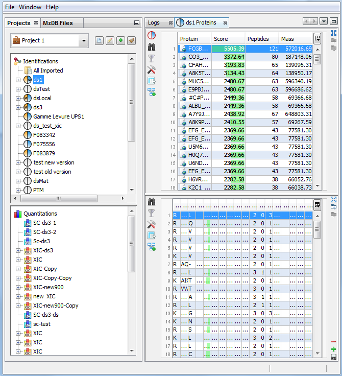
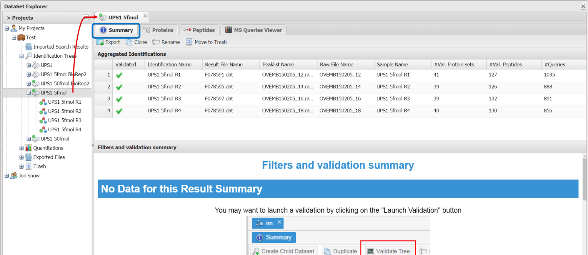
To display data of a Search Result:
- right click on a Search Result
- click on the menu “Display Search Result >” and on the sub-menu “MSQueries” or “PSM” or “Proteins”
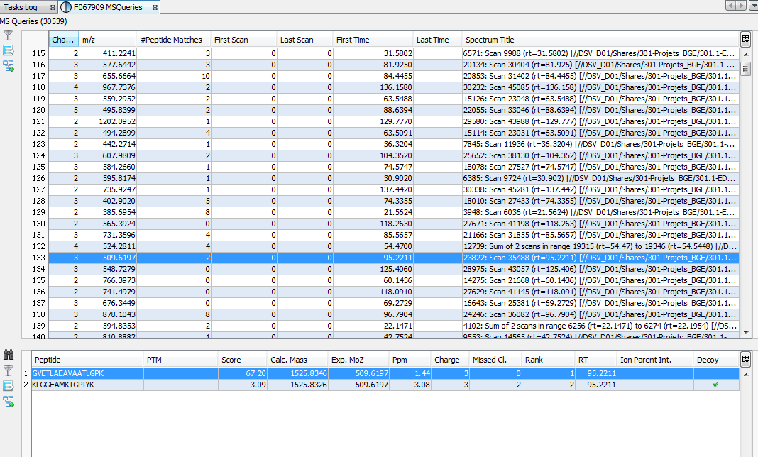
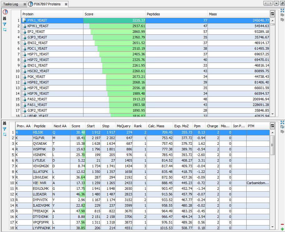
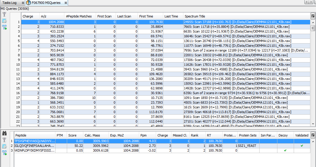
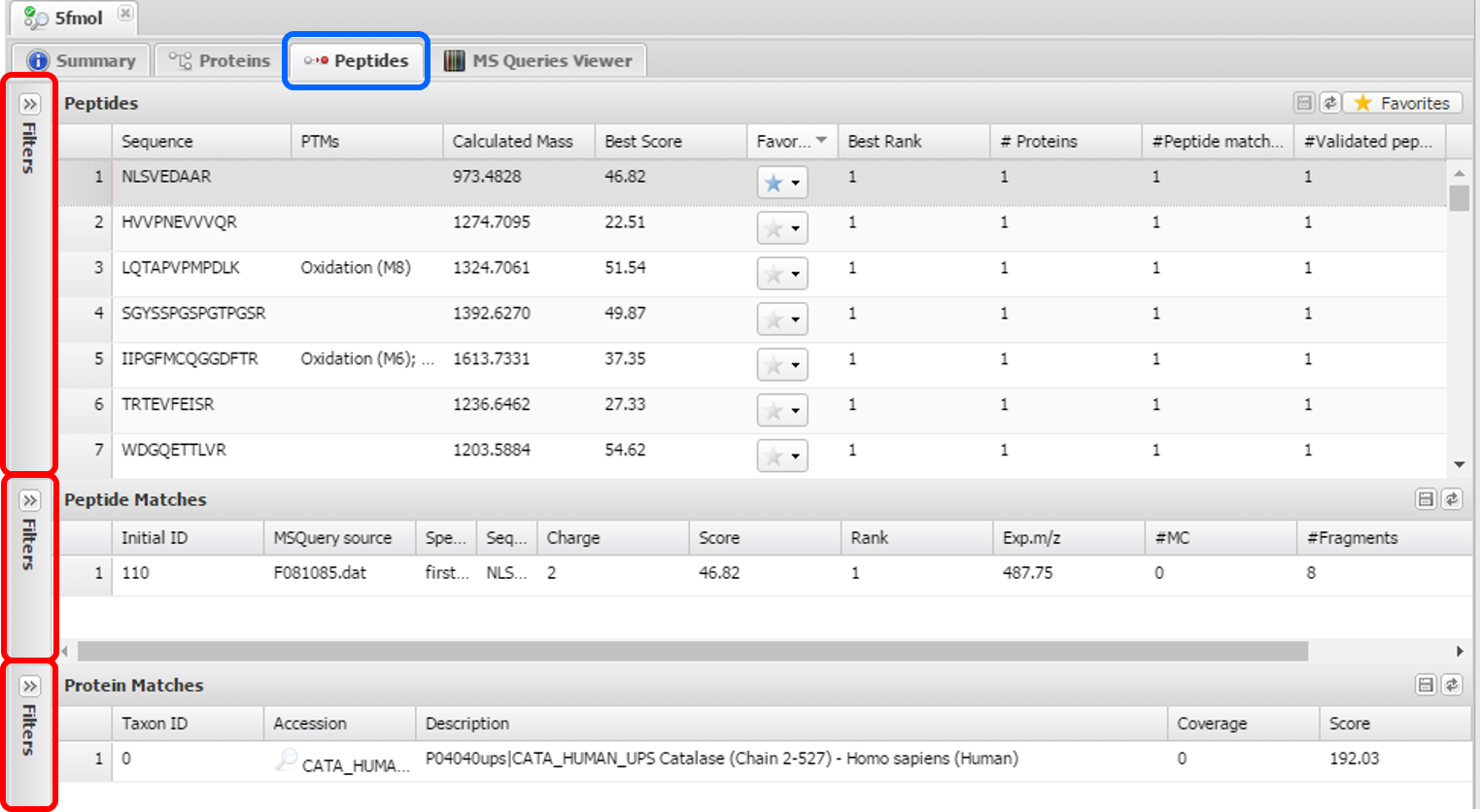
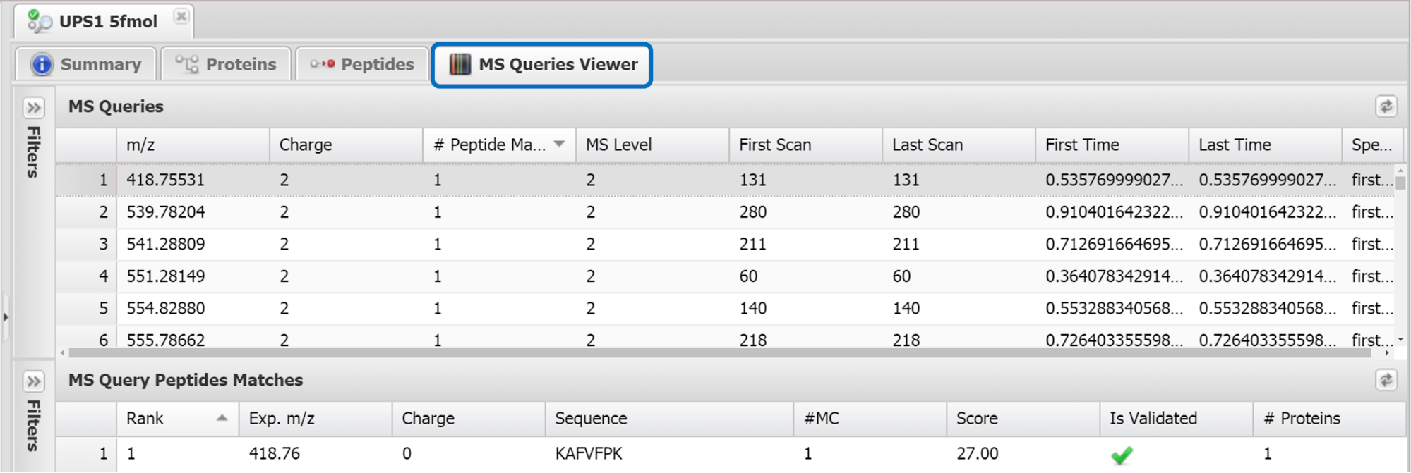
If you click on MSQueries sub-menu, you obtain this window:
Upper View: list of MSQueries.
Bottom Window: list of all Peptides linked to the current selected MSQuery.
Note: Abbreviations used are listed here
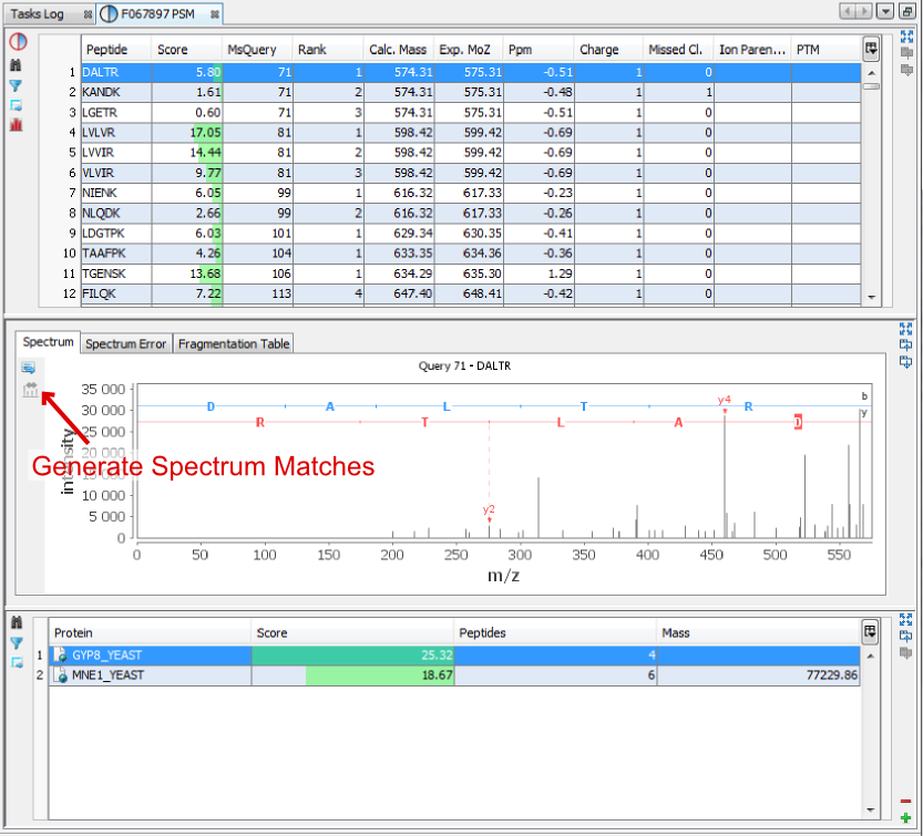
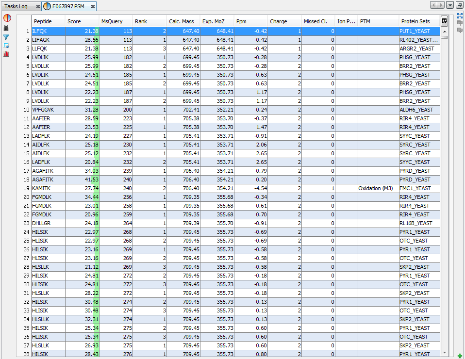
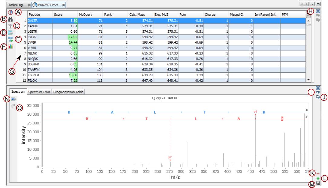
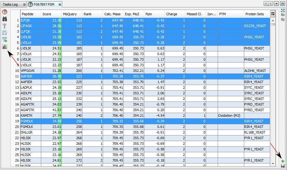
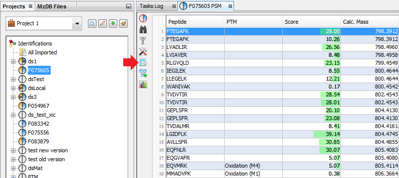
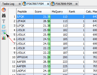
If you click on PSM sub-menu, you obtain this window:
Upper View: list of all PSM/Peptides.
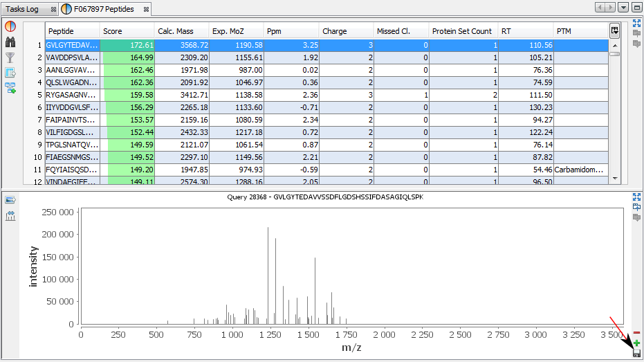
Middle View: Spectrum, Spectrum Error and Fragmentation Table of the selected PSM. If no annotation is displayed, you can generate Spectrum Matches by clicking on the according button
Bottom Window: list of all Proteins containing the currently selected Peptide.
Note: Abbreviations used are listed here
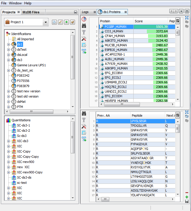
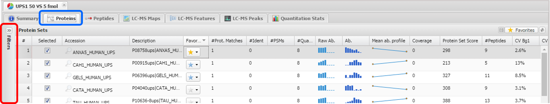
If you click on Proteins sub-menu, you obtain this window:
Upper View: list of all Proteins
Bottom View: list of all Peptides for the selected Protein.
Note: Abbreviations used are listed here
To display data of an Identification Summary:
- right click on an Identification Summary
- click on the menu “Display Identification Summary >” and on the sub-menu “MSQueries”, “PSM”, “Peptides”, “Protein Sets”, “PTM Protein Sites” or “Adjacency Matrix”
If you click on MSQueries sub-menu, you obtain this window:
Upper View: list of MSQueries.
Bottom Window: list of all Peptides linked to the current selected MSQuery.
Note: Abbreviations used are listed here
If you click on PSM sub-menu, you obtain this window:
Note: Abbreviations used are listed here
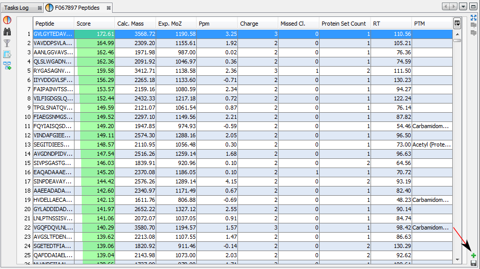
If you click on Peptides sub-menu, you obtain this window:
Upper View: list of all Peptides
Middle View: list of all Protein Sets containing the selected peptide.
Bottom Left View: list of all Proteins of the selected Protein Set
Bottom Right View: list of all Peptides of the selected Protein
Note: Abbreviations used are listed here
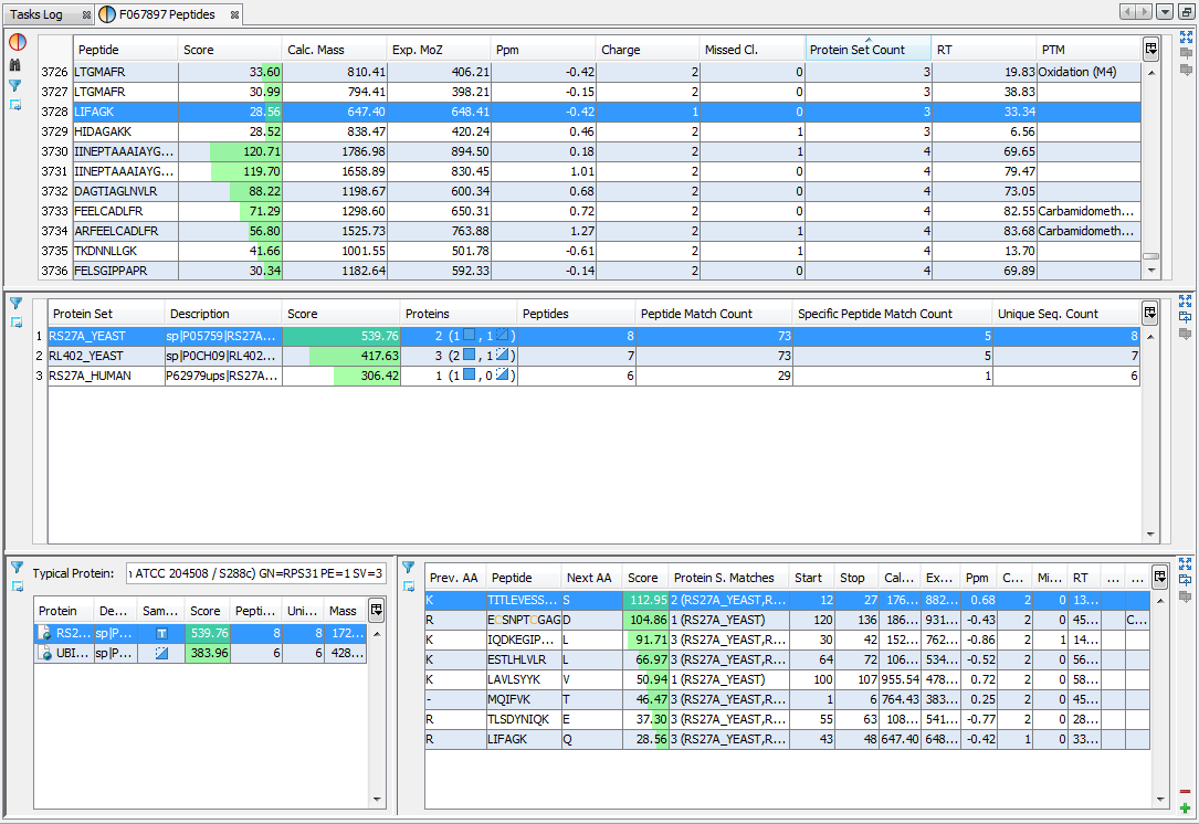
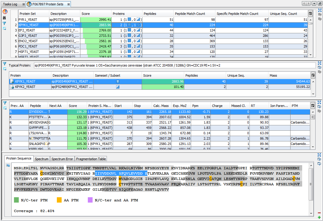
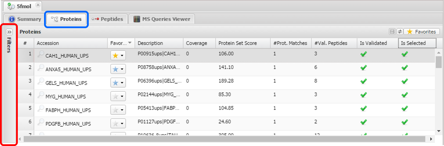
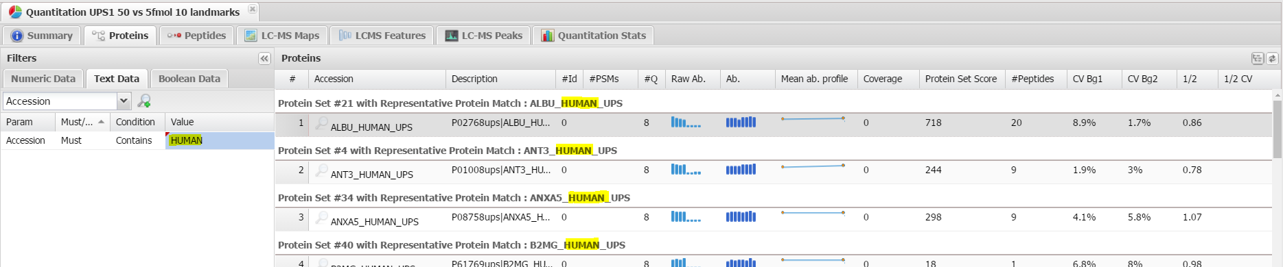
If you click on Protein Sets sub-menu, you obtain this window:
View 1 (at the top): list of all Protein Sets
Note: In the column Proteins, 8 (2, 6) means that there are 8 proteins in the protein set : 2 in the sameset, 6 in the subset.
View 2: list of all Proteins of the selected Protein Set.
View 3: list of all Peptides of the selected Protein
View 4: Protein Sequence of the previously selected Protein and Spectrum of the selected Peptide. Other tabs display Spectrum, Spectrum Error and Fragmentation Table.
Note: Abbreviations used are listed here
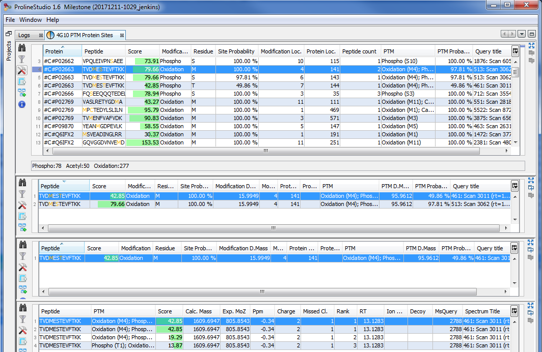
If you click on PTM Protein Sites sub-menu, you obtain this window:
WARNING: This windows will be filled in only if you have first run “Identify PTM Sites” from the dataset menu.
View 1 (at the top): This view lists all PTM Protein Sites (PTM on Protein at specific location) by displaying best PSM for current site.
View 2: For selected PTM Protein Site, list all peptides ( which matches. Best PSM for each peptide is displayed.
View 3: For selected peptide in View 2, display all associated PSMs.
View 4: For selected PSM in View 3, display all PSMs of same MSQuery.
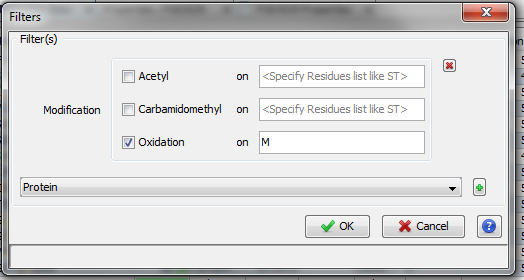
The user can filter on PTM Modification (by choosing Modification in filters list).
In the following example, the user keeps only Oxidation on residue M. I it possible to specify no residue to accept all, or to specify a list of residues.
View 4: Protein Sequence, Spectrum, Spectrum Error, Fragmentation Table and Spectrum Values
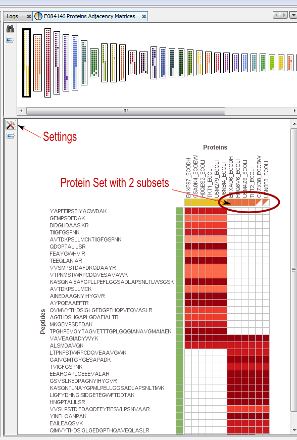
If you click on Adjacency Matrix sub-menu, you obtain this window:
View 1: All the matrices. Each matrix correspond of a cluster composed of linked Proteins/Peptides.
Note: use the Search tool to display an Adjacency Matrix for a particular Protein or Peptide
View 2: The currently selected matrix.
In the example, you can see two different protein sets which share only two peptides.
Thanks to the settings you can hide proteins with exactly the same peptides.
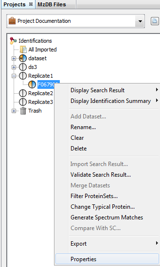
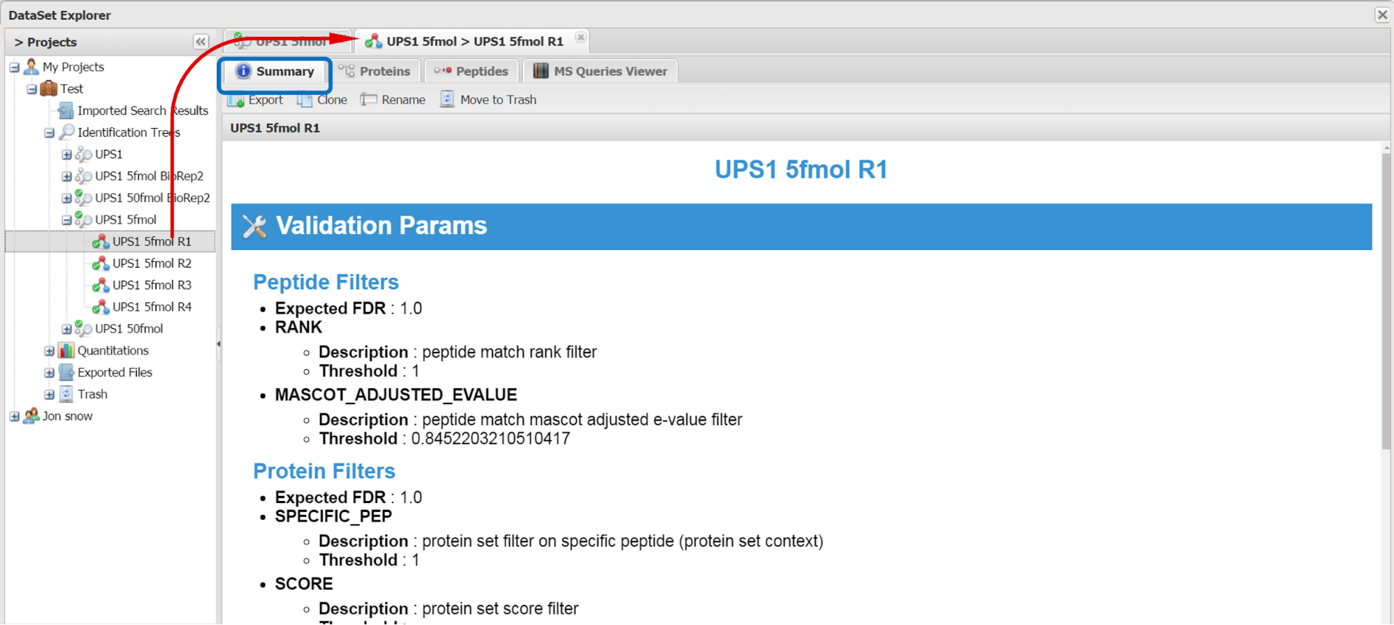
To display properties of a Search Result or Identification Summary:
Note: it is possible to select multiple Search Results/Identification Summaries to compare the values.
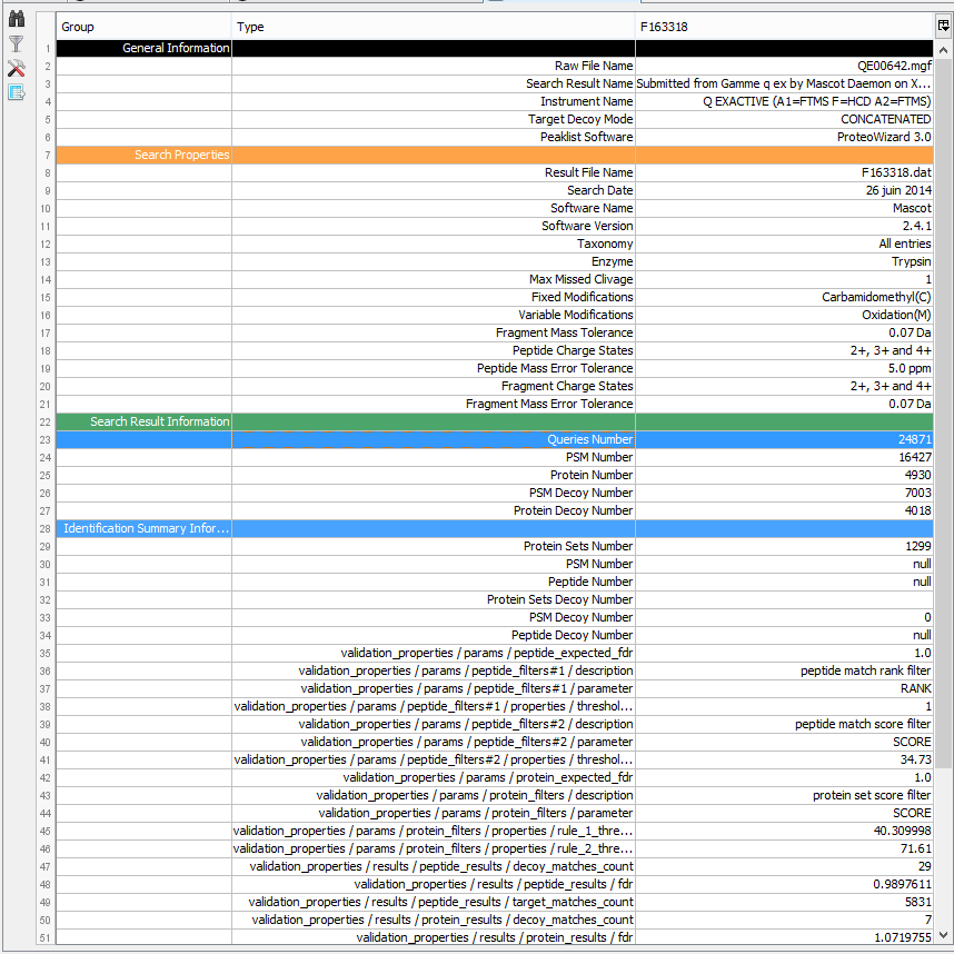
Property window opened:
General Information: Various information on the analysis (instrument name, peaklist software…)
Search Properties: Information extracted from the Result File (date, software version, search settings...)
Search Result Information: Amount of Queries, PSM and Proteins in the Search Result.
Identification Summary Information: Information obtained after validation process
Note 1: Validation parameters are tagged with “validation_properties / params”
Note 1: Validation results are tagged with “validation_properties / results”
Sql Ids: Database ids related to this item
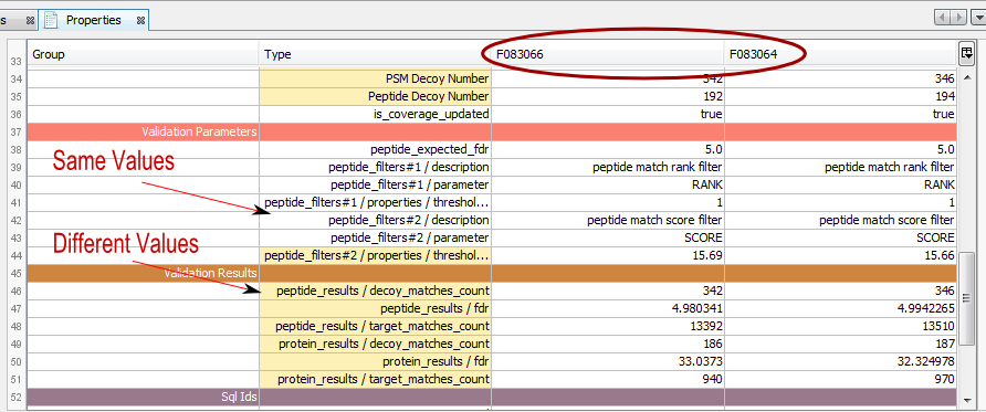
Property window opened with multiple Identification summaries selected:
The color of the type column indicate if the values are the same (white) or different (yellow).
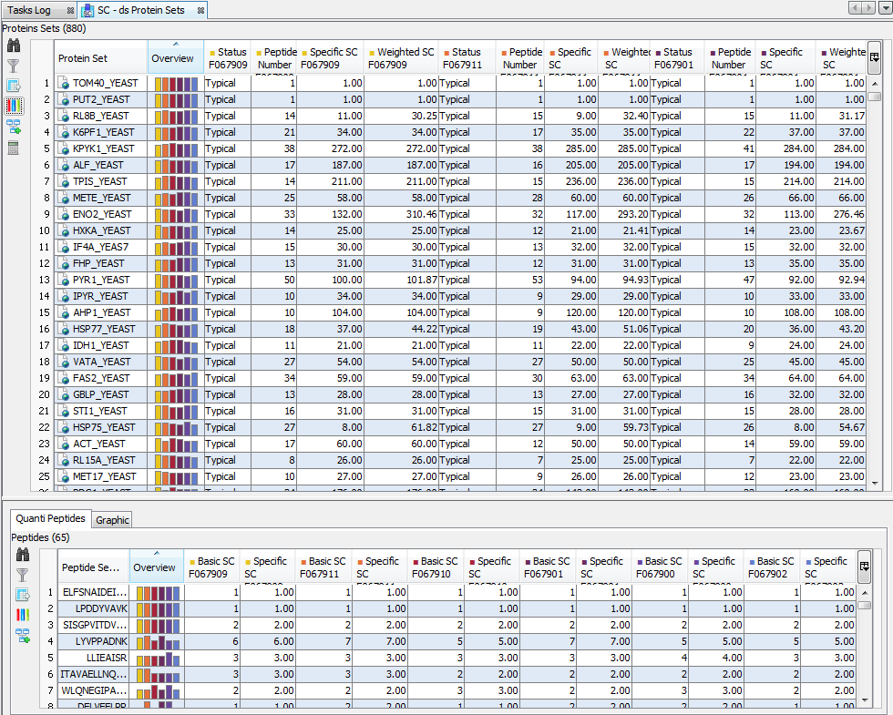
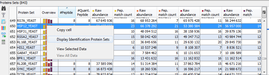
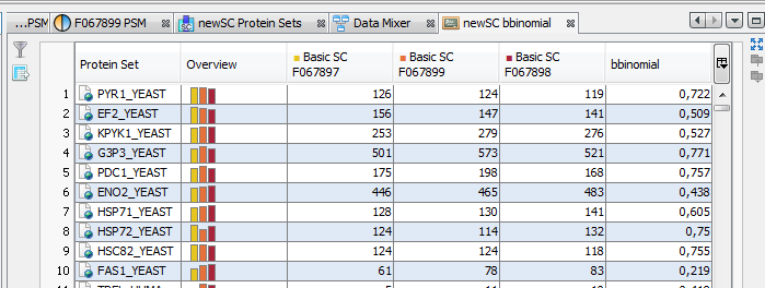
You can display a generated Spectral Count by using the right mouse popup.
To have more details about the results, see spectral_count_result
The overview is based by default on the weighted spectral count values. (Note: if you sort on the overview column, the sort is based on max (value-mean (values))/mean (values). So, you will obtain the most homogenous and confident rows first)
For each dataset, are displayed:
- status ( typical, sameset, / )
- peptide numbers
- the basic spectral count
- the specific spectral count
- the weighted spectral count (by default)
- the selection level
By clicking on the “Column Display Button” , you can choose the information you want to display or change the overview.
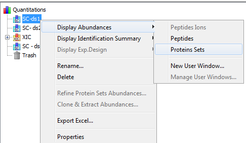
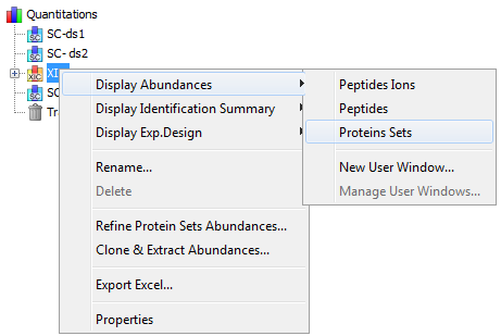
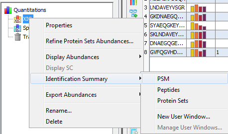
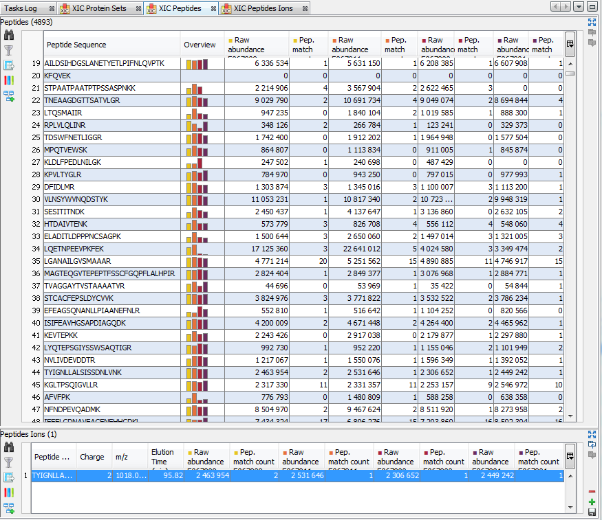
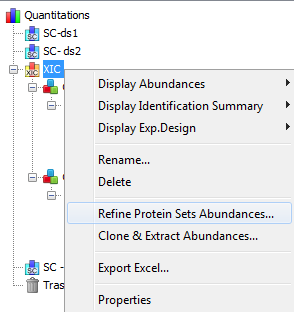
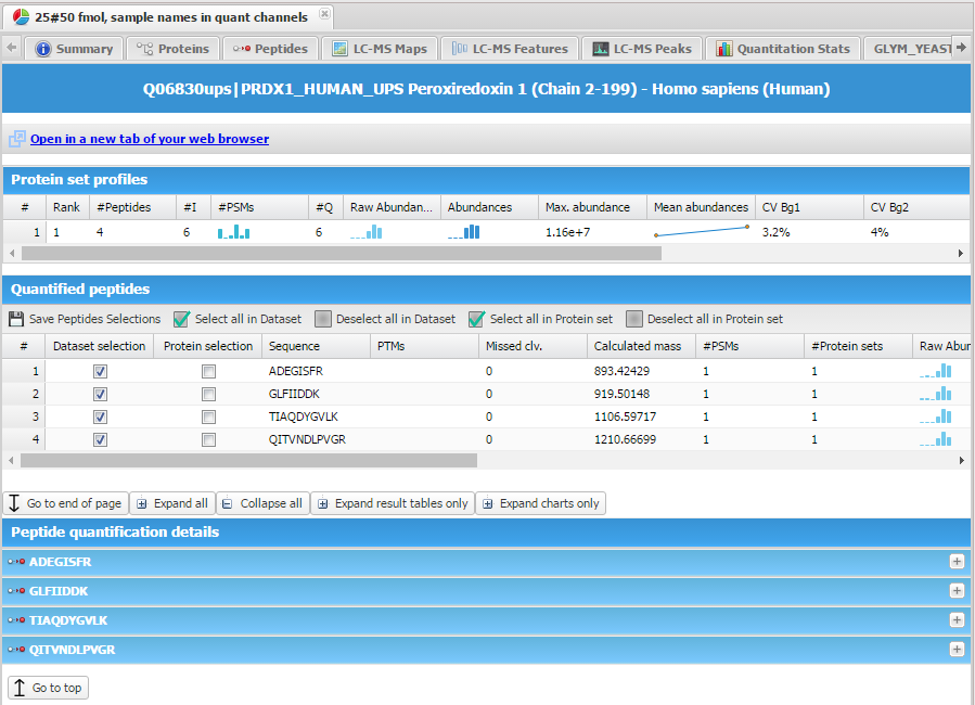
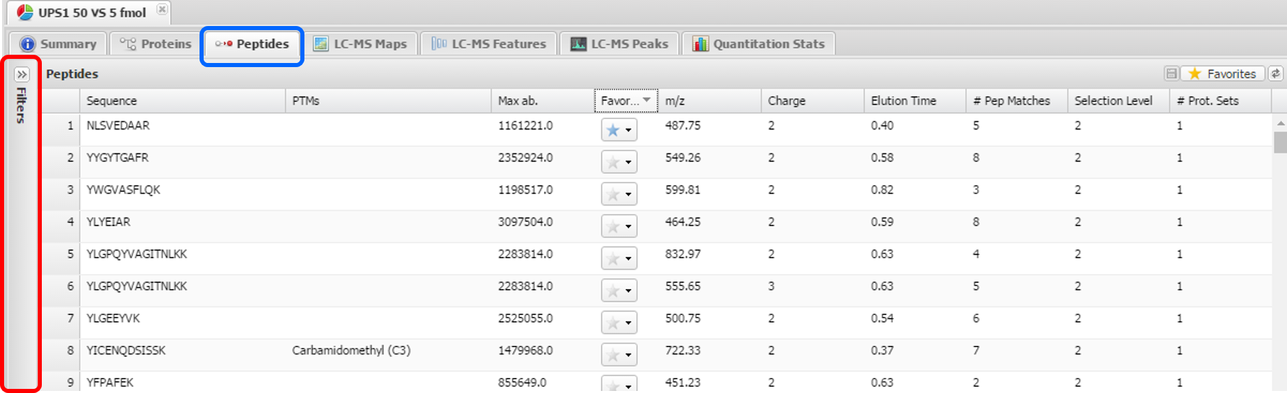
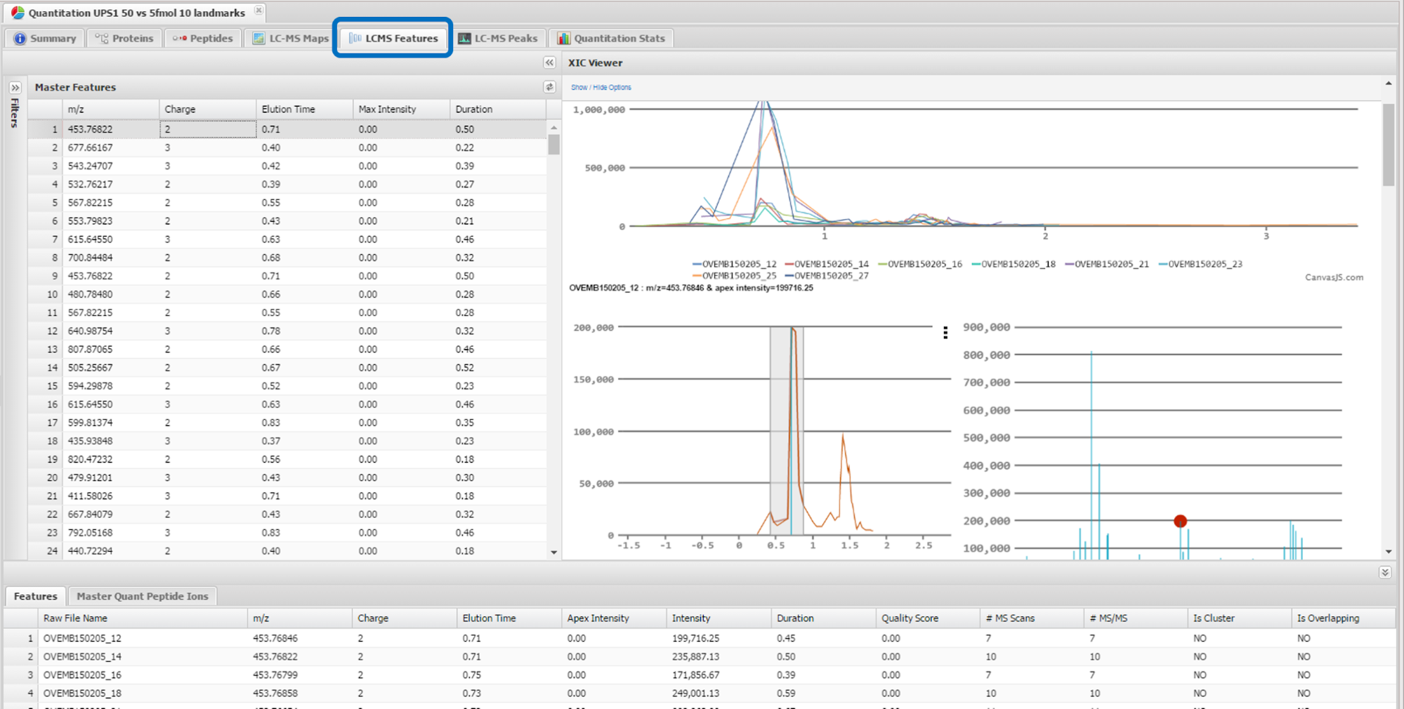
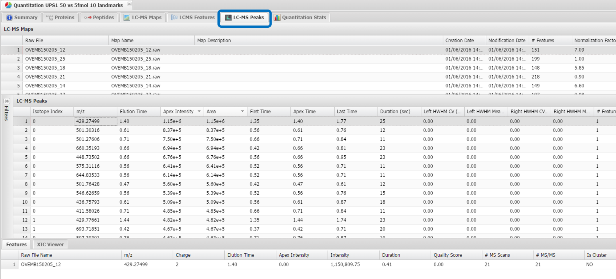
To display a XIC, right click on the selected XIC node in the Quantitation tree, and select “Display Abundances”, and then the level you want to display:
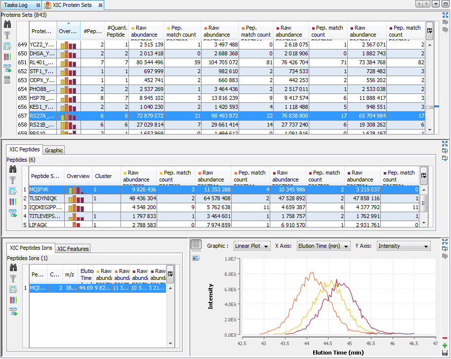
By clicking on “Display Abundances” / “Protein Sets”, you can see all quantified protein sets. For each quantified protein set, you can see below all peptides linked to the selected protein set and peptides Ions linked to the selected peptide. For each peptide Ion, you can see the different features and the graph of the peakels in each quantitation channel.
The overview is based by default on the abundances values.
Note: if you sort on the overview column, the sort is based on max (value-mean (values))/mean (values). So, you obtain the most homogenous and confident rows first.
For each quantitation channel, are displayed:
- the raw abundance
- the peptide match count (by default)
- the abundance (by default)
- the selection level
By clicking on the “Column Display Button” , you can choose the information you want to display or change the overview.
To display the identification protein Set view, click right on the selected protein Set and select “Display Identification Protein Sets” menu in the popup.
You can also display the identification summary result from the popup menu in the quantitation tree:
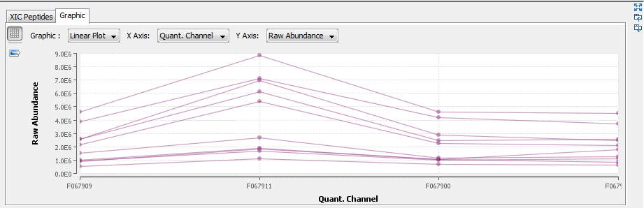
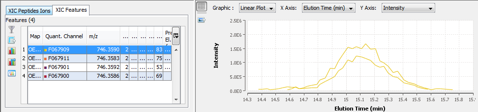
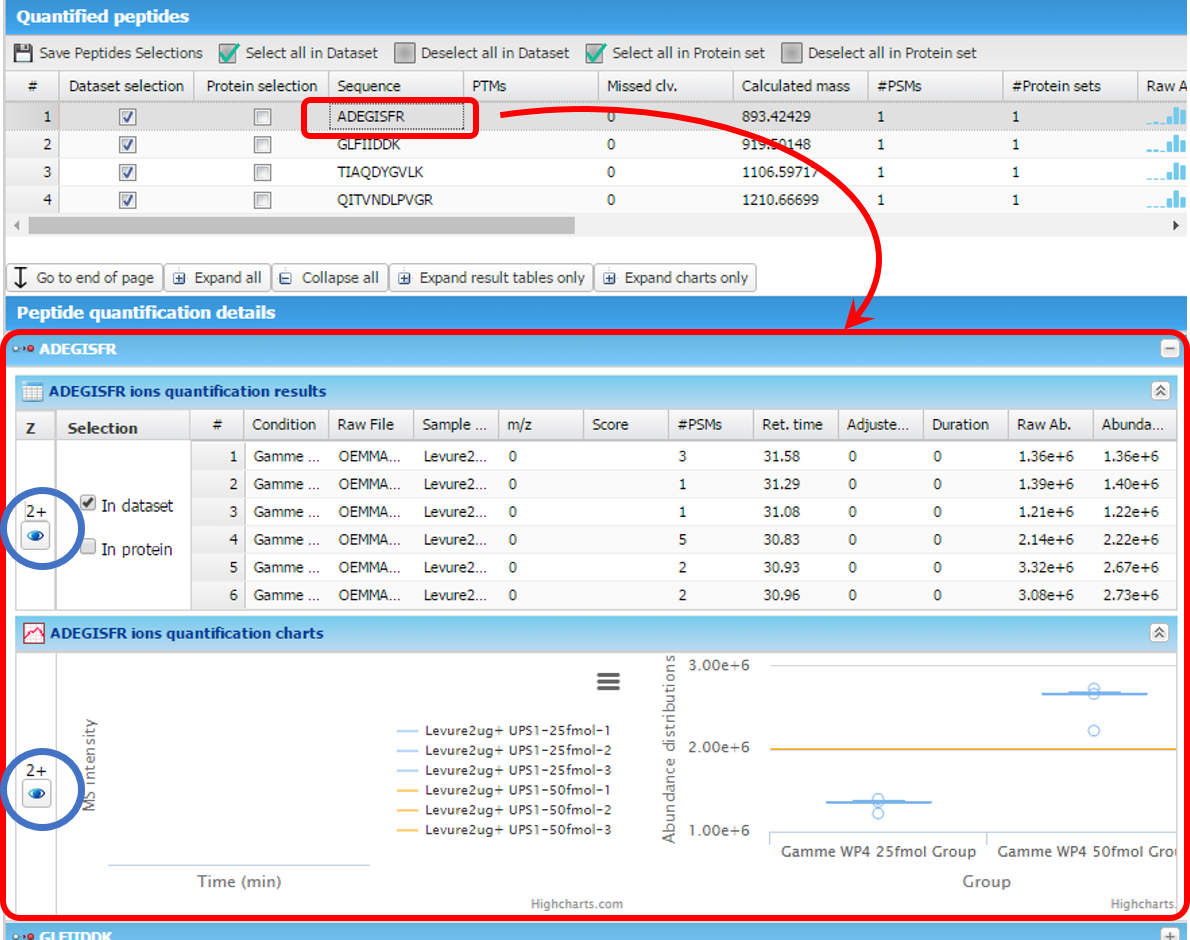
A graph allows you to see the variations of the abundance (or raw abundance) of a peptide in the different quantitation channels:
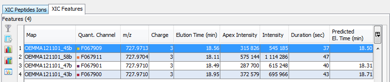
You can see the different features in the different quantitation channels and the graph of the peakels:
By clicking on you can display either:
- the peaks of isotope 0 in all quantitation channels
- all isotopes for the selected quantitation channel:
By clicking on you can see the chromatograms of the features and their first time scan and last time scan in mzScope. For more details see the mzScope section.
By clicking on “Display Abundances“ / “Peptides”, you can see:
- identified and quantified Peptides
- non identified but quantified peptides
- identified but not quantified peptides (linked to a quantified protein)
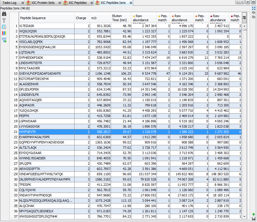
By clicking on “Display Abundances” / “Peptides Ions”, you can see:
- all identified and quantified Peptides Ions
- non identified but quantified peptides Ions
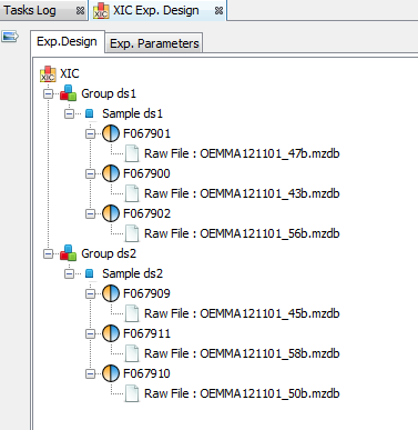
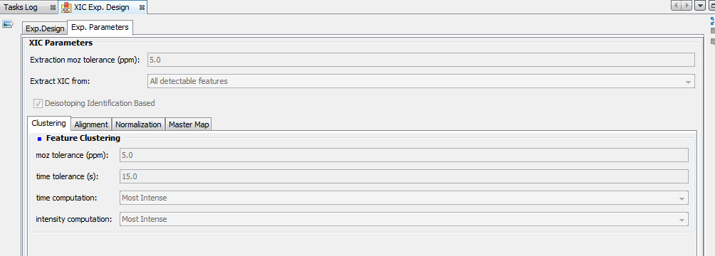
By clicking on “Exp. Design > Parameters”, you can see the experimental design and the parameters of the selected XIC.
If you have launched the refinement of the protein sets abundances on the XIC, you can also display the refinement parameters.
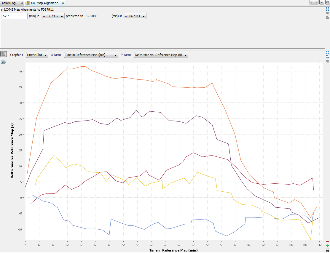
By clicking on “Exp. Design > Map Alignment”, you can see the map of the variation of the alignment of the maps compared to the map alignment of the selected XIC. You can also calculate the predicted time in a map from an elution time in another map.
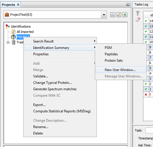
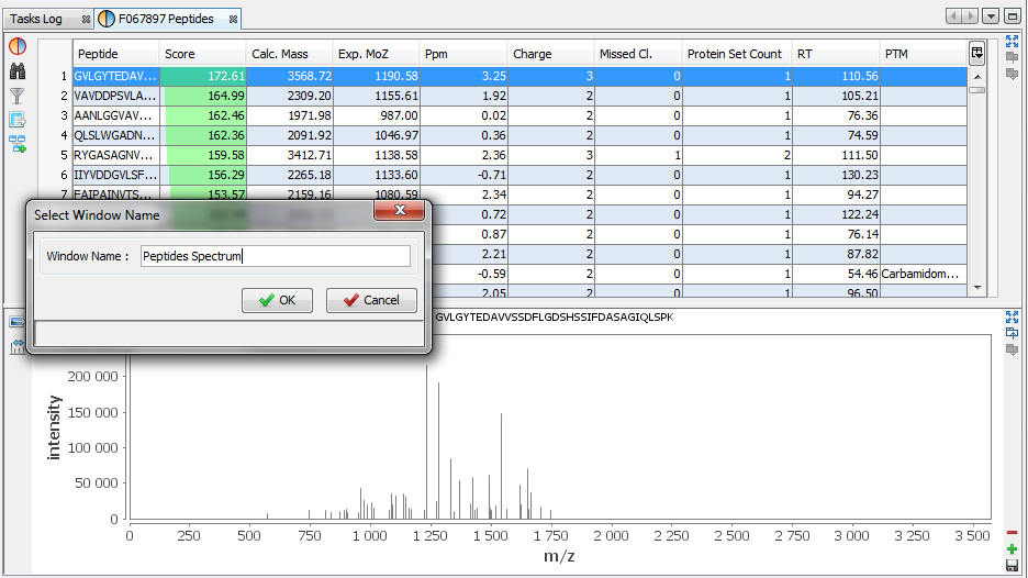
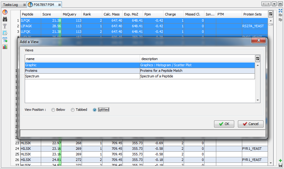
You can lay out your own user window with the desired views.
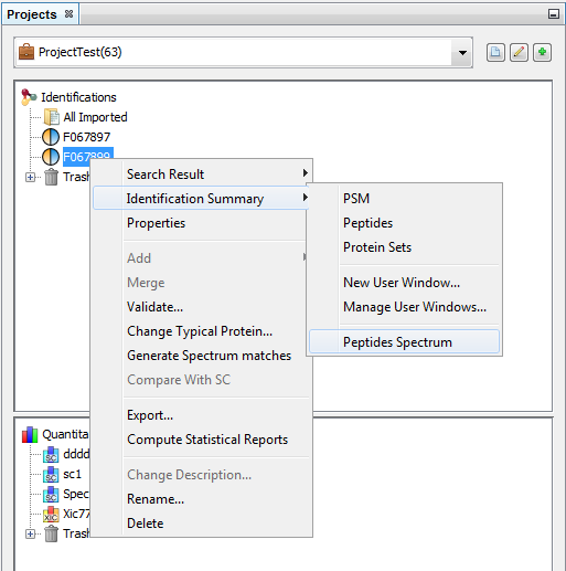
You can do it from an already displayed window, or by using the right click mouse popup on a dataset like in the following example (Use menu “Search Result>New User Window…” or “Identification Summary>New User Window…”)
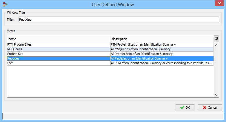
In the example, the user has clicked on “Identification Summary>New User Window…” and selects the Peptides View as the first view of his window.
You can add other views by using the '+' button.
In this example, the user has added a Spectrum View and he saves his window by clicking on the “Disk” Button.
The user selects 'Peptides Spectrum' as his user window name
Now, the user can use his new 'Peptides Spectrum' on a different Identification Summary.
A: Display Decoy Data.
B: Search in the Table. (Using * and ? wild cards)
C: Filter data displayed in the Table
D: Export data displayed in the Table
E: Send to Data Analyzer to compare data from different views
F: Create a Graphic : histogram or scatter plot
G: Right click on the marker bar to display Line Numbers or add Annotations/Bookmarks
H: Expands the frame to its maximum (other frames are hidden). Click again to undo.
I: Gather the frame with the previous one as a tab.
J: Split the last tab as a frame underneath
K: Remove the last Tab or Frame
L: Open a dialog to let the user add a View (as a Frame, a Tab or a splitted Frame)
M: Save the window as a user window, to display the same window with different data later
N: Export view as an image
O: Generate Spectrum Matches
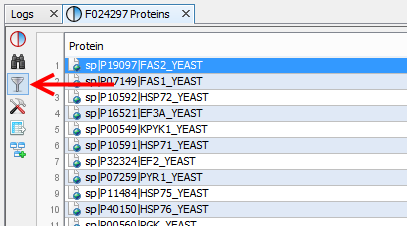
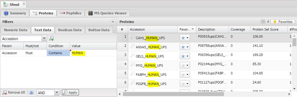
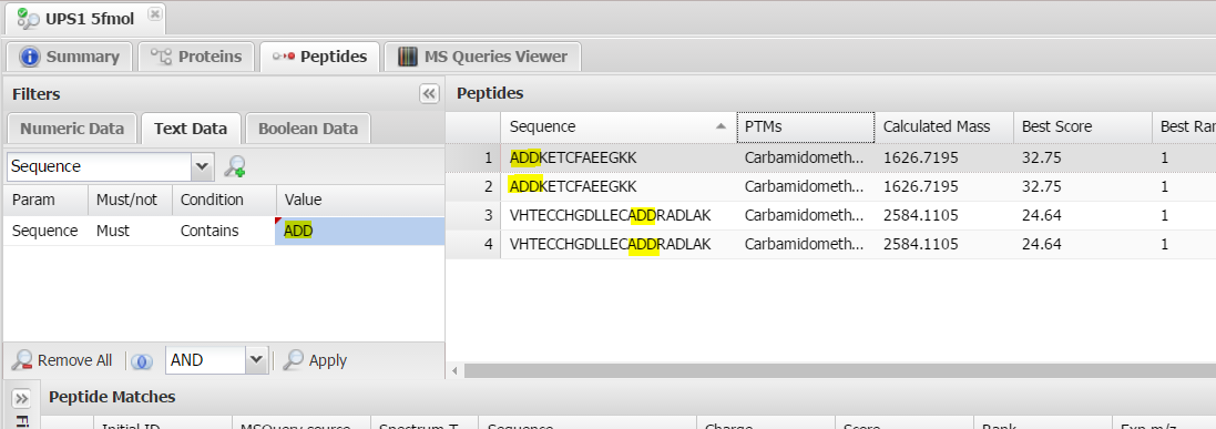
You can filter data displayed in the different tables thanks to the filter button at the top right corner of a table.
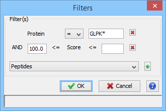
When you have clicked on the filter button, a dialog is opened. In this dialog you can select the columns of the table you want to filter thanks to the “+” button.
In the following example, we have added two filters:
- one on the Protein Name column (available wildcards are * to replace multiple characters and ? to replace one character)
- one on the Score Column (Score must be at least 100 and there is no maximum specified).
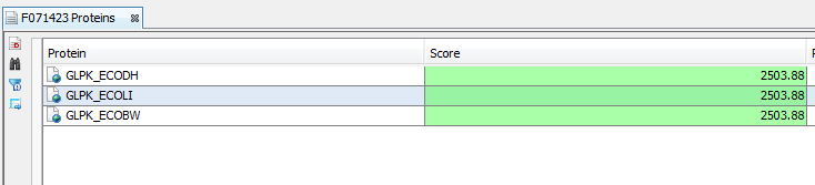
The result is all the proteins starting with GLPK (correspond to GLPK*) and with a score greater or equal than 100.
Note: for String filters, you can use the following wildcards: * matches zero or more characters, ? matches one character.
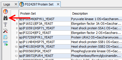
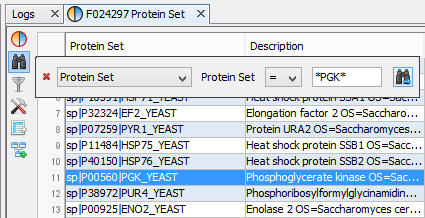
In some tables, a Search Functionality is available thanks to the search button at the top right corner.
When you have clicked on the search button, a floating panel is opened. In this panel you can select the column searched and fill in the searched expression, or the value range.
For searched expressions, two wild cards are available:
In the following example, the user search for a protein set whose name contains “PGK”.
You can do an incremental search by clicking again on the search button of the floating panel, or by pressing the Enter key.
There are two ways to obtain a graphic from data:
If you have clicked on the '+' button, the Add View Dialog is opened and you must select the Graphic View
A: Display/Remove Grid toggle button
B: Modify color of the graphic
C: Lock/Unlock incoming data. If it is unlocked, the graphic is updated when the user apply a new filter to the previous view (for instance Peptide Score >= 50) If it is locked, changing filtering on the previous view does not modify the graphic.
D: Select Data in the graphic according to data selected in table in the previous view.
E: Select data in the table of the previous view according to data selected in the graphic.
F: Export graphic to image
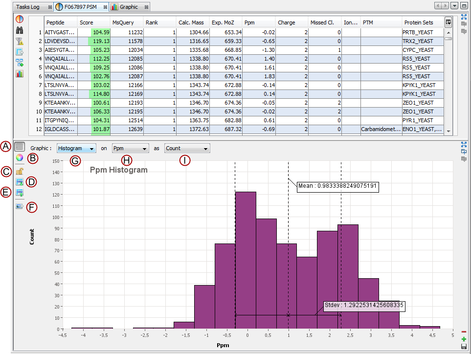
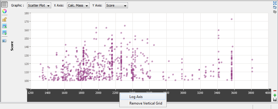
G: Select the graphic type: Scatter Plot / Histogram
H/I: Select data used for X / Y axis.
It is possible to select linear or log axis by right clicking on an axis.
Zoom in: Press the right mouse button and drag to the right bottom direction. A red box is displayed. Release the mouse button when you have selected the area to zoom in.
Zoom out: Press the right mouse button and drag to the left top direction. When you release the mouse button, the zooming is reset to view all.
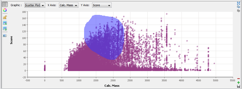
Select: Press the left mouse button and drag the mouse to surround the data you want to select. When you release the button, the selection is done. Or left click on the data you want to select. It is possible to use Ctrl key to add to the previous selection.
Unselect: Left click on an empty area to clear the selection.
You can run a Quality Control on any Search Result. It consists in a transversal view of the imported data: rather than visualising the results per PSM or Proteins, results are sorted according to the score, charge state...
Choose the menu option:
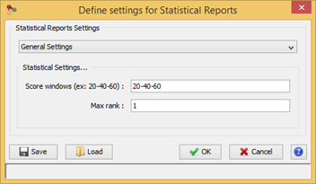
Configure some settings before launching the process
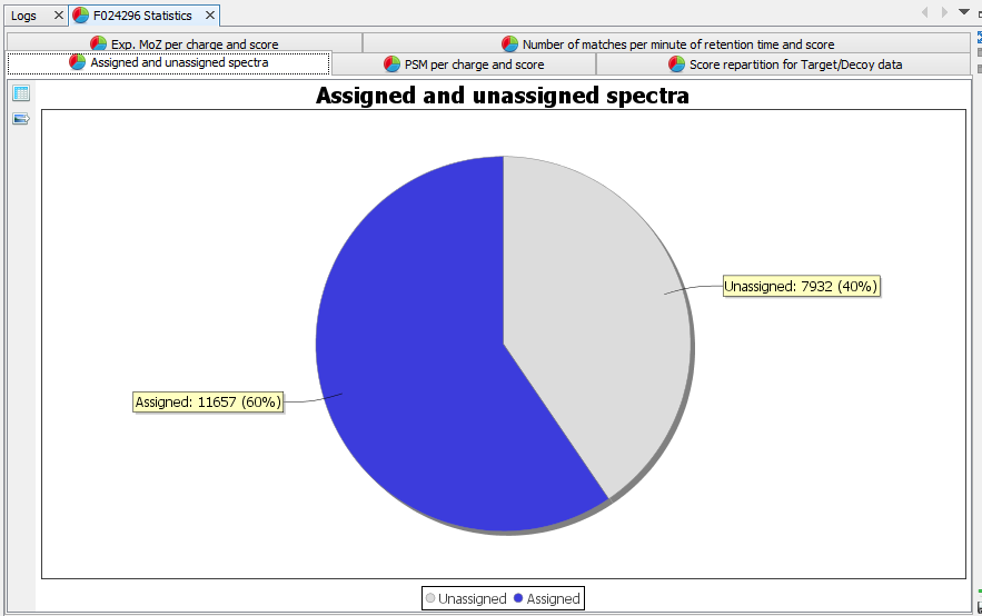
The report will appear in a matter of seconds (depending of the amount of data to be processed). You will get the following tabs:
Assigned and unassigned spectra: Pie chart presenting the ratio of assigned spectra | |
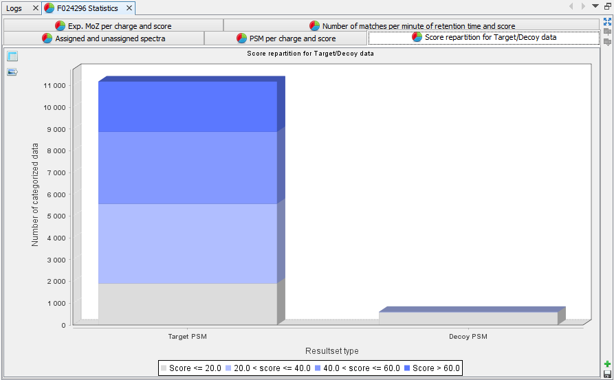
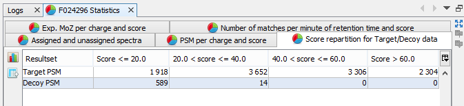
Score repartition for Target/Decoy data: Histogram presenting the amount of PSM per group of score, separating target and decoy data | |
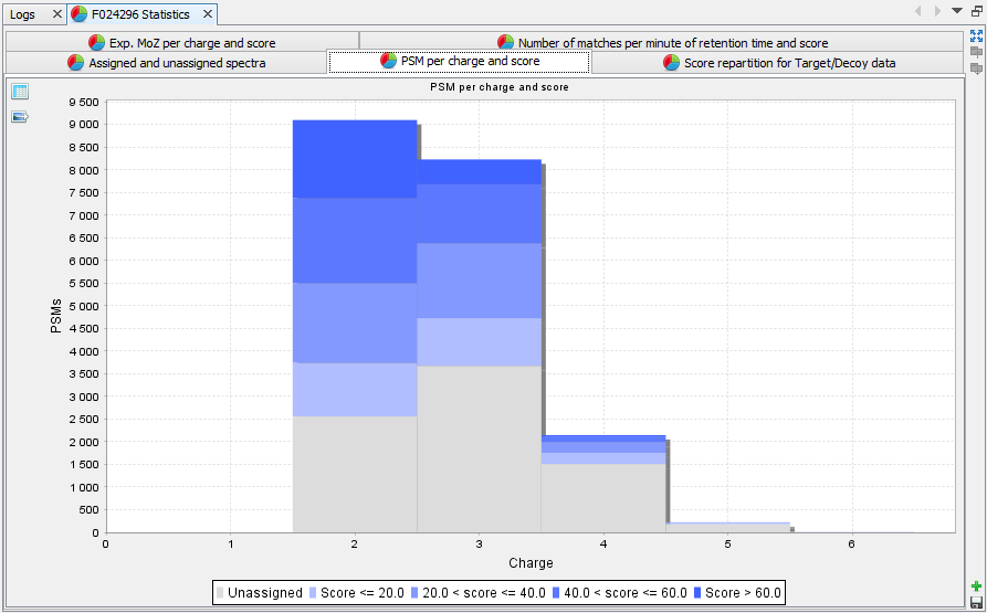
PSM per charge and score: Histogram presenting the amount of PSM per group of score and charge state | |
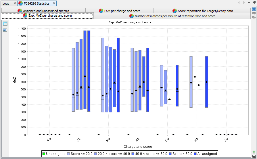
Experimental M/z per charge and score: Box plot presenting M/z information for each category of score and charge state | |
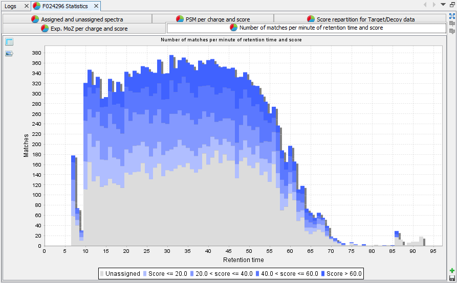
Number of matches per minute of RT and score: histogram presenting the amount of PSM per score and retention time. This view is only calculated when retention time is available. | |
Each graph is also available in a table view |
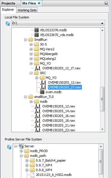
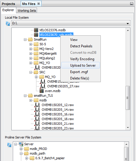
In order to facilitate different actions on Ms Files, Proline Studio contains an homonym tab providing the end user with a view over his local and a remote file system, called Local File System and Proline Server File System respectively. Furthermore, through an appropriate popup menu, a series of actions can take place on the encountered .mzdb and .raw files, including among others the:
Apart from the popup menu supported functionality, since Proline Studio 1.5, conversions and uploads can be triggered via drag and drop mechanism. In this context, an .mzdb file’s drag and drop triggers a file upload while dragging and dropping a .raw file from the local site to the remote one provokes a conversion proceeded by its respective upload.
As mentioned earlier, after selecting a number of files, the user can either drag and drop them inside the remote site, or use the popup menu as shown in the following screenshot. It is important to precise that both approaches are not compatible with a selected group consisting of different file types.
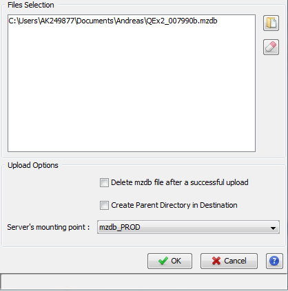
As we can see, clicking on upload opens a dedicated dialog packing a series of uploading options:
Furthermore, the dialog permits us to change the synthesis of the selected group by adding or removing supplementary .mzdb files. While the last option is significant as it defines the final destination, the first two, the creation of the parent file and the deletion after the successful upload are considered to be an aid to keep the destination folder well organized. Clicking OK on the dialog will make it disappear dispatching at the same time an uploading batch, consisting of an uploading task for each .mzdb file. Uploading tasks, as all tasks that are dispatched within Proline Studio, can be monitored at the Logs tab.
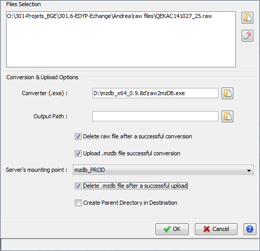
In the same way, when the user desires to convert and upload a raw file, he or she, can either drag and drop it on the Remote Site view, or use the respective dialog through the popup menu.
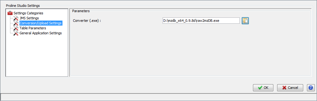
As we can see, this dialog follows a very similar format and logic compared to the one used by the upload dialog. Apart from the already seen settings that regard the upload itself, we can distinguish a few more, purely regarding the process of conversion. The two most important options are the selected converter and the output path. The latter one corresponds to the directory where the .mzdb file will be created when raw2mzDB.exe will finish its cycle. It must be noted that if a conversion has never taken place before, there is a very high probability that the converter’s option is blank, unless a default converter has been defined through the general settings dialog. Furthermore, this value among others, is saved or updated everytime the user clicks on OK, so that the latter one does not have to fill in all the fields when he or she wants to perform a conversion.
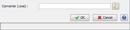
Dragging and dropping a .raw file at the remote view follows a little bit different approach. Since we cannot upload a raw file to the server, the drag and drop action basically correspond to a .raw file conversion followed by the respective upload. Given the fact that when dragging a file no dialog appears, the conversion is based on the default converter set in the general settings window. If such setting has not yet taken place, a popup dialog will appear demanding the selection of a converter to be used. The latter one also updates the aforementioned field in the general settings.
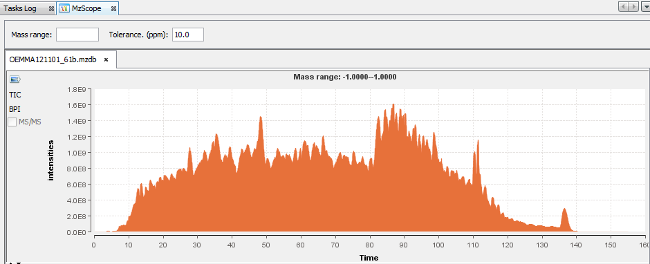
By default, the TIC chromatogram is displayed. You can click on “BPI” to see the best peak intensity graph.
By clicking in the graph, you can see below the scan at the selected time.
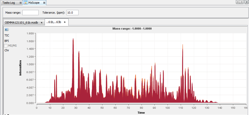
You can choose to display 2 or more chromatograms on the same graph, by selecting 2 files and clicking on “View Data”
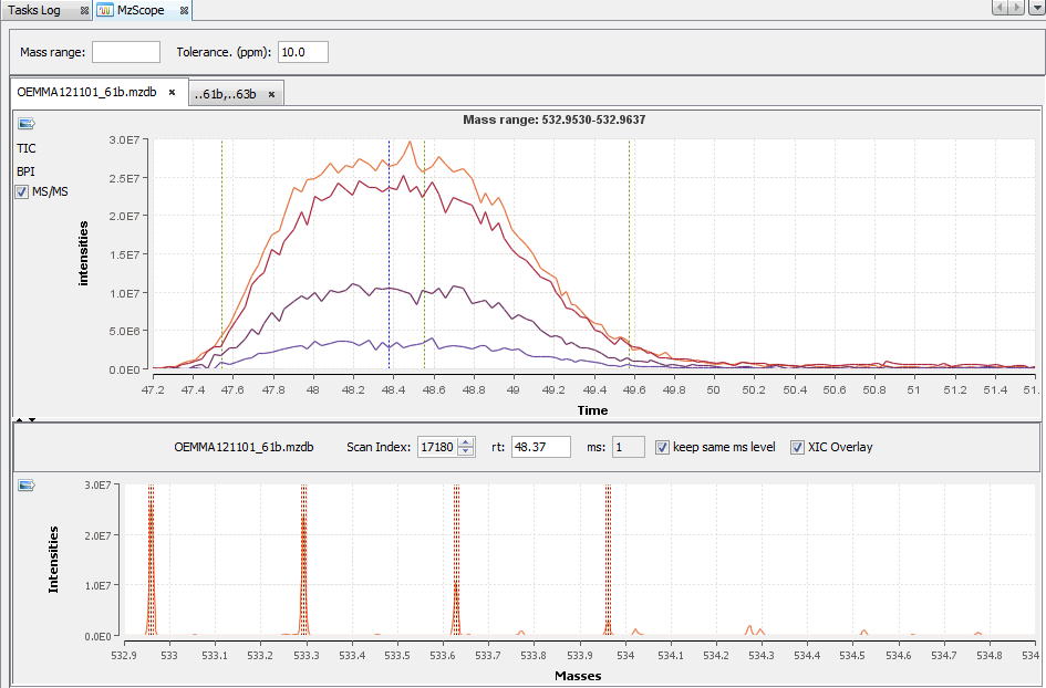
You can extract a chromatogram at a given mass by entering the specified value in the panel above.
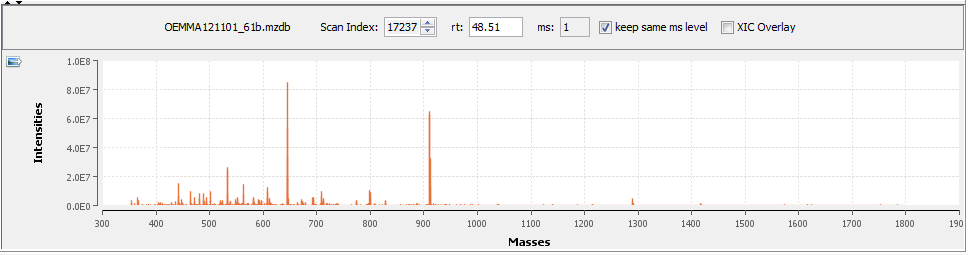
You can navigate through the scans
- by increasing or decreasing the scan Ids
- by entering a retention time
- by clicking the keys arrows on the keyboard (Ctrl+Arrows to keep the same ms level)
By double clicking on the scan, the corresponding chromatogram is displayed above (The Alt key or the check box “XIC overlay” allows you to overlay the chromatograms in the same graph).
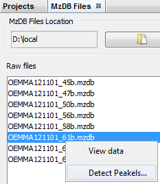
By selecting a file, you can click on “Detect Peakels” in the popup menu.
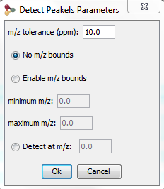
A dialog allows you to choose the parameters of the peakels detection: the tolerance and eventually a range of m/z, or a m/z value:
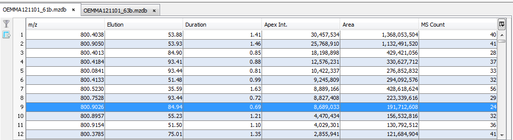
The results are displayed in a table:
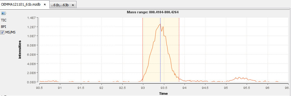
You can double-click (or through the popup menu) on a row to display the peakel in the corresponding raw file:
There are many ways to do an export:
- Export a Table using the export button (supported formats: {xlsx, xls, csv})
- Export data using Copy/Paste from the selected rows of a Table to an application like Excel.
- Export all data corresponding to an Identification Summary, XIC or Spectral Count
- Export an image of a view
- Export Identification Summary data into Pride (ProteomeXchange) format.
- Export Identification Summary spectra list.
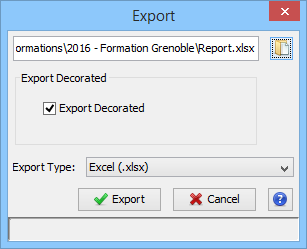
To export a table, click on the Export Button at the left top of a table.
An Export Dialog is opened, you can select the file path for the export and the format of the export (supported formats: {xlsx, xls, csv}).
In case that the selected format is either .xls or .xlsx, the user has now the ability to maintain in his exported excel document any rich text format elements (color, font weight etc.) apparent on the original table in Proline Studio. Choice is done using the checkbox shown on the following screenshot.
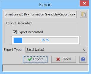
To perform the export, click on the Export Button. The task can take a few seconds if the table has a lot of rows and so a progress bar is displayed.
Note: the following feature regarding the export will be functional in the next release of Proline Studio.
To copy/Paste a Table:
- Select rows you want to copy
- Press Ctrl and C keys at the same time
- Open your spreadsheet editor and press Ctrl and V keys at the same time to paste the copied rows.
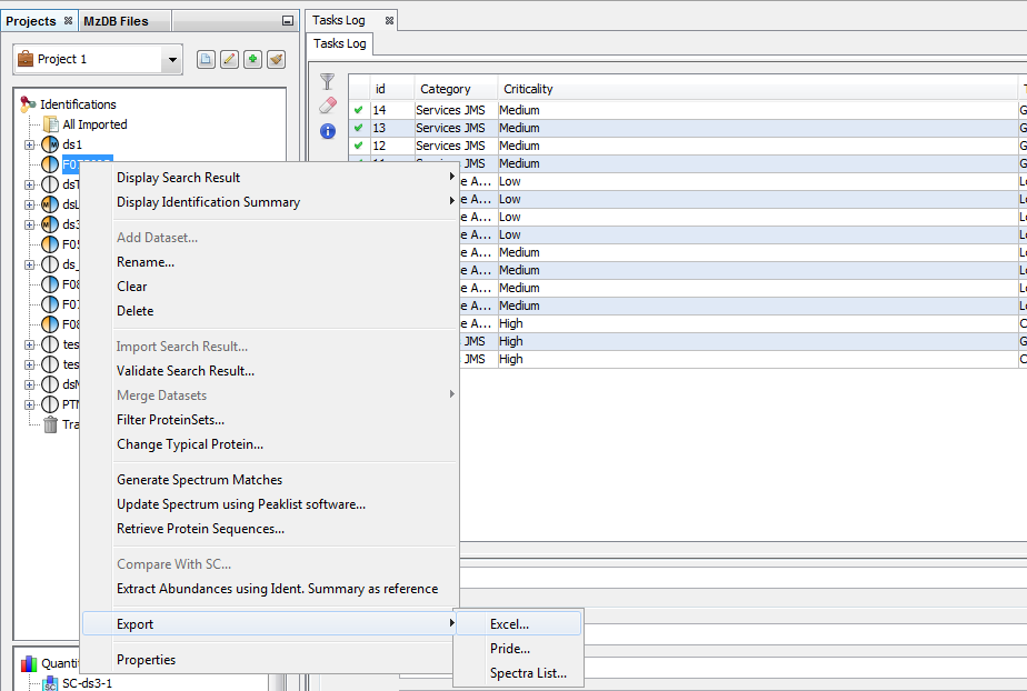
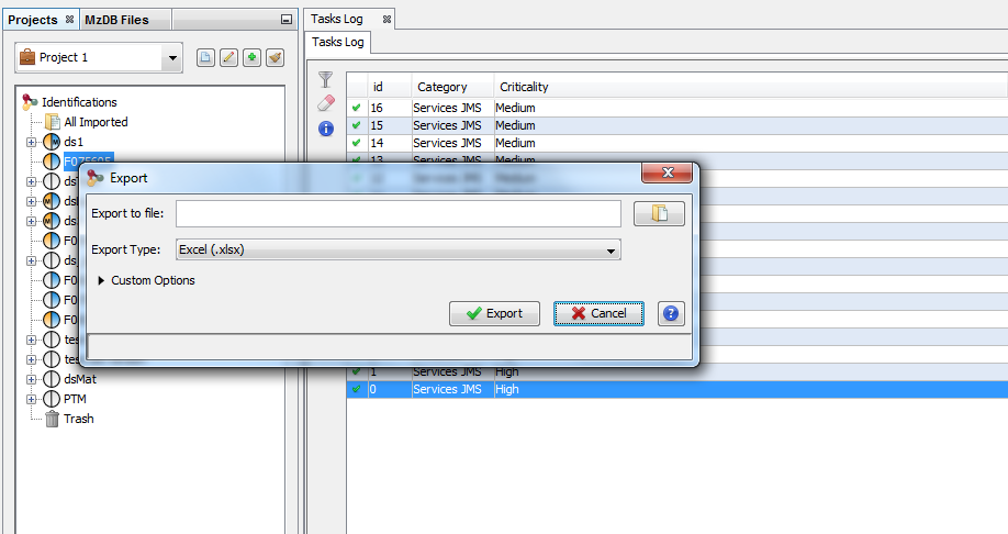
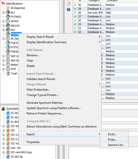
To Export all data of an Identification Summary, a XIC or a Spectral Count, right-click on the dataset to open the contextual menu and select the “Export” menu and then “Excel...” sub-menu.
You can also export multiple dataset simultaneously, if they have the same type (Identification Summary or XIC or Spectral Count).
An Export Dialog is opened, you can select the file path and the type of the export : Excel (.xlsx) or Tabulation separated values (.tsv).
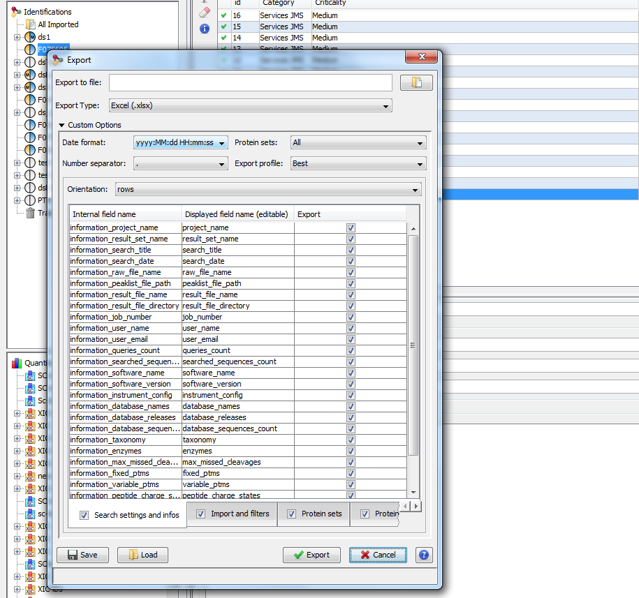
You can export with the default parameters or perform a custom export. To enable custom export, click on the tickbox located on the right of the dialog:
Custom export allows a number of parameters in addition to the file format to be chosen:
You can enable/disable individual sheets, rename them, rename individual fields and move then up and down, disable them. You can also save your own configuration and load it later on, and even share it with colleagues. (configuration file stored locally).
Description of exported file is available here.
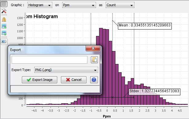
To export a graphics, click on the Export Image Button at the left top of the image.
An Export Dialog is opened, you can select the file path for the export and the type of the export. You can export any images in PNG format or SVG format. SVG format produces a vector image that can be edited and resized afterwards.
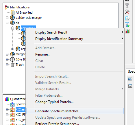
Note: Before exporting data to Pride format, all spectrum matches should have been generated. To do so, right click on the dataset and select “Generate Spectrum Matches”.
To export all data of an Identification Summary into Pride (ProteomeXchange compatible) format, you must right click on the dataset to open the contextual popup and select the “Export > Pride…” Menu.
Some additional information could be specified (some of them are required, those with a *) in the displayed dialogs.
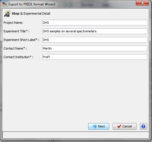
a. Experimental Details: Specify Project and Experiment name and contact
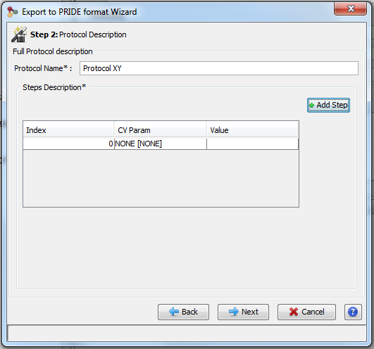
b. Protocol Description: Specify a name for the Protocol Description. Add at least one Step for the description by clicking on “Add Step” button.
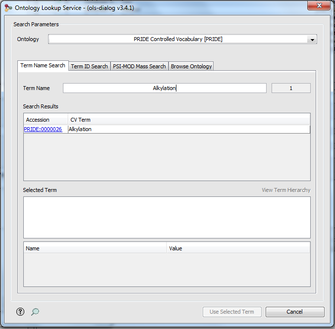
An ontology search dialog will be opened to help getting protocol step description
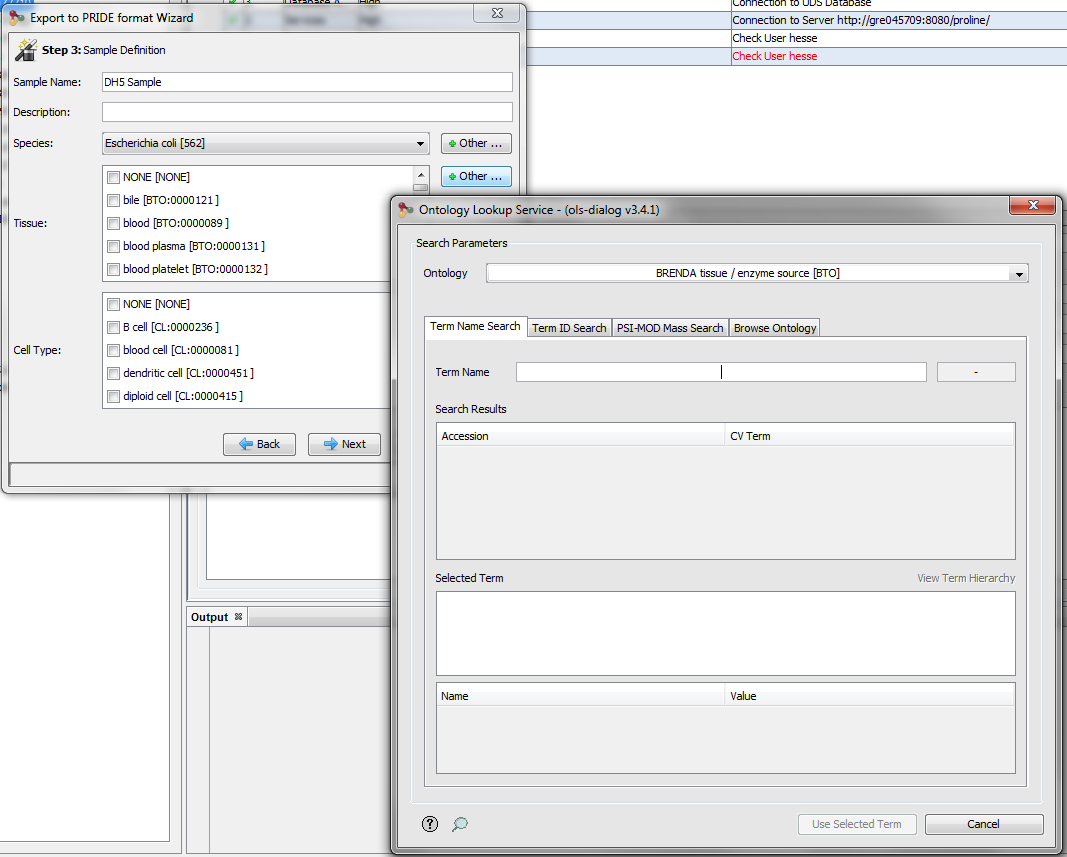
c. Sample Description: Specify a sample name and description. Species, Tissue and Cell Type is specified using Controlled Vocabulary. If desired data is not listed, you can click on the “other…” button to search through complete ontology.
To export valid PSM Spectra from an Identification Summary or from a XIC Dataset. The exported tsv file is compatible with Peakview.
Note: all Spectrum Matches must be generated first.
When importing a Search Result in Proline, user can view PSM with their associated Spectrum but by default no annotation is defined. User can generate (and save) this information
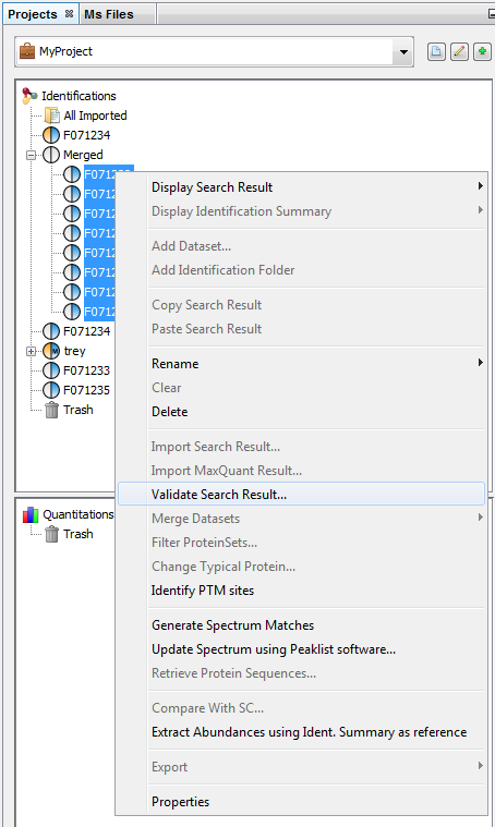
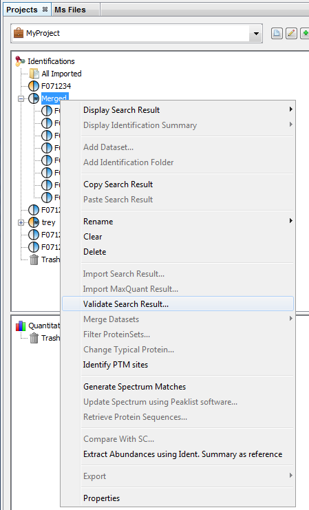
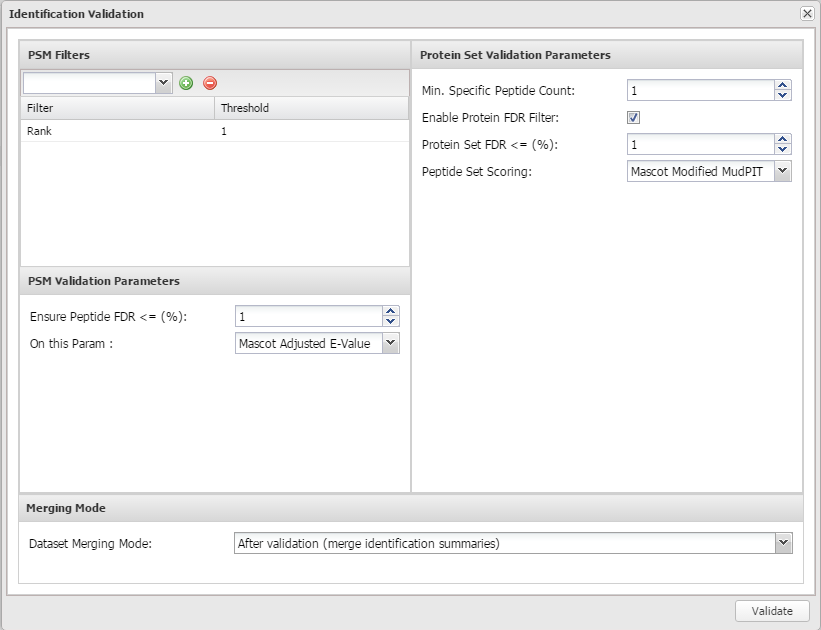
See description of Validation Algorithm.
It is possible to validate identification Search Result or merged ones. In latest case, the filters and validation threshold can be propagated to child Search Results.
To validate a Search Result:
- Select one or multiple Search Results to validate
- Right Click to display the popup
- Click on “Validate…” menu
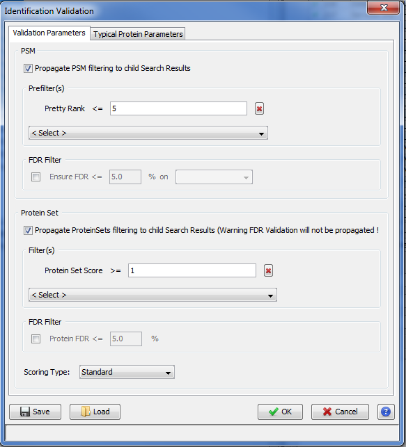
In the Validation Dialog, fill the different Parameters (see Validation description):
- you can add multiple PSM Prefilter Parameters ( Rank, Length, Score, e-Value, Identity p-Value, Homology p-Value) by selecting them in the combobox and clicking on Add Button '+'
- you can ensure a FDR on PSM which will be reached according to the variable selected ( Score, e-Value, Identity p-Value, Homology p-Value,… )
- you can add a Protein Set Prefilter on Specific Peptides.
- you can ensure a FDR on protein Sets.
Note: FDR can be used only for Search Results with Decoy Data.
If you choose to propagate to child Search Result, specified prefilters will be used as defined. For the FDR Filter, it is the threshold found by the validation algorithm which will be used for childs, as a prefilter.
In the second tab, you can define rules for choosing the Typical Protein of a Protein Set by using a match string with wildcards ( * or ? ) on Protein Accession or Protein Description. (see Change Typical Protein of Protein Sets).
Validating a Search Result can take some time. While it is not finished, the Search Results are shown greyed with an hourglass over them. The tasks are displayed as running in the “Tasks Log Dialog”.
When the validation is finished, the icon becomes orange and blue. Orange part correspond to the Identification Summary. Blue is for the Search Result part.
See description of Protein Sets Filtering.
The protein sets windows are not updated after filtering Protein Set. You should close and reopen the window
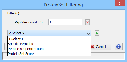
To filter Protein sets of Identification Summaries:
- Select one or multiple Identification Summaries to filter
- Right Click to display the popup
- Click on “Filter ProteinSets…” menu
you can add multiple filters (Specific Peptides, Peptide count, Peptide sequence count, Protein Set Score) by selecting them in the combobox and clicking on Add Button '+'
Once the filtering is done, you will have to open new protein sets window in order to see modification.
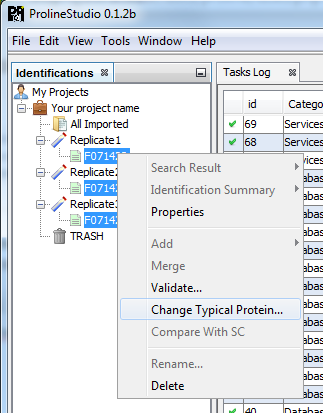
The protein sets windows are not updated after changing Typical Protein. You should close and reopen the window
To change the Typical Protein of the Protein Sets of an Identification Summary:
- Select one or multiple Identification Summaries
- Right Click to display the popup
- Click on “Change Typical Protein…” menu
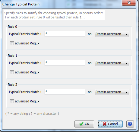
You can set the choice for the Typical Protein of Protein Sets by using a match string with wildcards (* or ?) on Protein Accession or Protein Description.
For Advanced user, a fully regular expression could be specified. In this case, check the corresponding option.
Three rules could be specified. They are applied in priority order, i.e. if no protein of a protein set satisfy the first rule, the second one is tested and so on.
The modification of Typical Proteins can take some time. During the processing, Identification Summaries are displayed grayed with an hourglass and the tasks are displayed in the Tasks Log Window
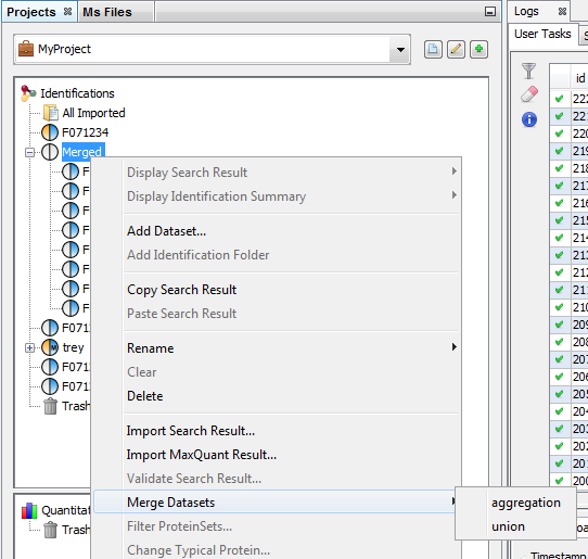
Merge can be done on Search Results or on Identification Summaries. In both case, you can specify if aggregation mode or union mode should be used. See description for Search Results merging and Identification Summaries merging
To merge a dataset with multiple Search Results:
- Select the parent dataset
- Right Click to display the popup
- Click on “Merge” menu
When the merge is finished, the dataset is displayed with an M in the blue part of the icon, indicating that the Merge has been done at a Search Result level.
If you merge a dataset containing Identification Summaries. The merge is done on an Identification Summary level. Therefore the dataset is displayed with an M in the orange part of the icon.
The purpose of the Data Analyzer is to easily do calculations/comparisons on data.
To open the data analyzer, you have two possibilities:
- you can use the dedicated button that you can find in the toolbar of all views. If you use this button, the corresponding data is directly sent to the data analyzer.
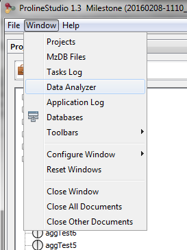
- you can use the menu “Window > Data Analyzer”
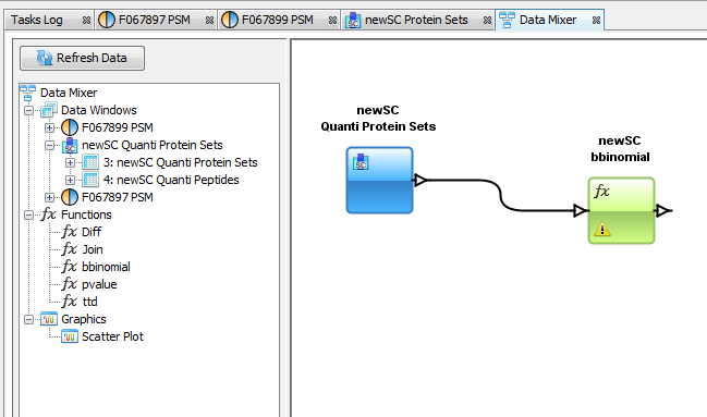
In the Data Analyzer view, you can access to all data views, to some functions and graphics. In the following example, we create a graph by adding by Drag & Drop the Spectral Count Data and the beta-binomial (BBinomial) function. Then we link them together.
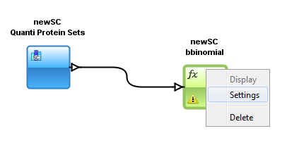
You have to specify the parameters of the BBinomial Function: right click on the function and select the “settings” menu
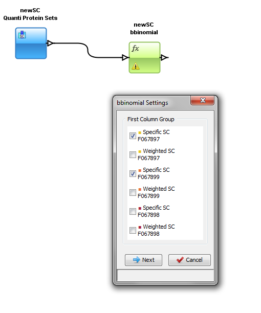
In the settings menu, select the two groups of columns on which you want to perform the BBinomial function. When the parameters are set, the calculation is started immediately and an hourglass icon is shown.
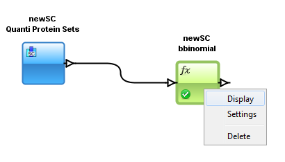
When the calculation is finished: the hourglass icon becomes a green tick, and the user can right click and select the “Display” menu to see the result.
This function is used by ProStar Macro to compute the FDR.
More information: http://bioconductor.org/packages/release/bioc/vignettes/Prostar/inst/doc/Prostar_UserManual.pdf
Join data of two tables according to selected key.
Perform a difference between two joined table data according to a selected key. When a key value is not found in one of the data source table, the line is displayed as empty. For numerical values a difference is done and for string values, the '<>' symbol is displayed when values are different.
Calibration Plot for Proteomics is described here: https://cran.r-project.org/web/packages/cp4p/index.html
bbinomial function is useful for Spectral Count Quantitations
This function is used by ProStar Macro. Two tests are available: Welch t-test and Limma t-test.
More information: http://bioconductor.org/packages/release/bioc/vignettes/Prostar/inst/doc/Prostar_UserManual.pdf
Columns filter, let the user remove unnecessary columns in a matrix. A combobox, with prefix and suffix of the columns, let you select multiple similar columns to filter then rapidly.
Rows filter function let the user filter some rows of a matrix according to settings on columns.
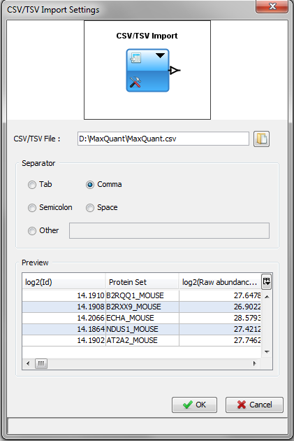
This module lets you import data from a CSV or TSV file. Then you can do calculations and display these data directly in Proline Studio.
The separator is automatically selected according to the csv file. But you can modify it.
The preview zone display the first lines of the file as it will be loaded.
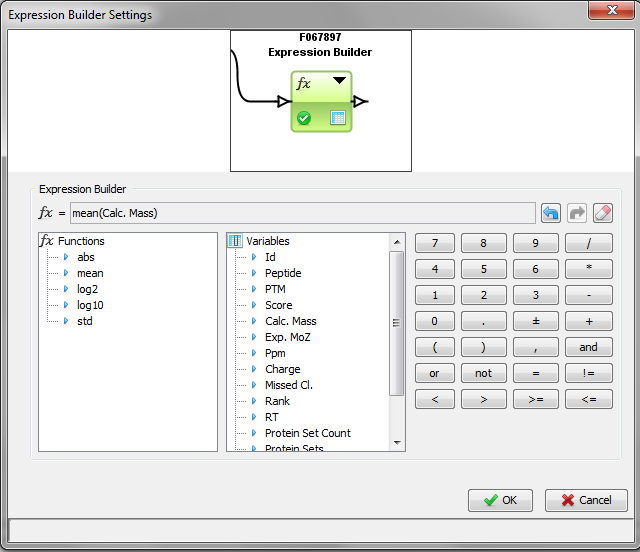
The expression builder let you create an expression with built-in functions or comparator and variables (columns from the linked matrix). In the example, we calculate the mean of a column in the matrix.S
This function is used by ProStar Macro to remove rows with too many missing quantitative values.
The available missing values algorithm are:
This function is used by ProStar Macro to impute missing values.
More information: http://bioconductor.org/packages/release/bioc/vignettes/Prostar/inst/doc/Prostar_UserManual.pdf
This function is used by ProStar Macro to normalize quantitative values.
More information on algorithms: http://bioconductor.org/packages/release/bioc/vignettes/Prostar/inst/doc/Prostar_UserManual.pdf
pvalue and ttd functions are useful for XIC Quantitations
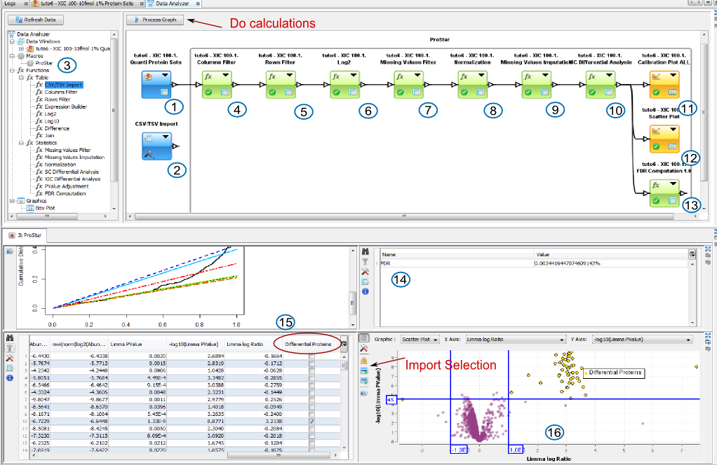
1 or 2: Add XIC Data to Data Analyzer from the Protein Set View or by importing data from a csv file.
3: Add Prostar Macro by a drag and drop and link XIC Data to the Macro. And do the calculation the by clicking on the button Process Graph.
During the process, the Data Analyzer will ask you settings for each function.
4: Filter unnecessary columns from your data if. Settings can be validated with no parameters if you don't need it.
5: Filter is needed only if you want to remove contaminants. Settings can be validated with no parameters if you don't need it.
6: Log is needed to log abundances (Data from Proline). For Data coming from MaxQuant, data is already logged.
7 to 13: follow the settings asked ( you can find some help in Prostar documentation, or information in corresponding functions.)
During the process, results will be automatically displayed:
14: FDR Result
15: Calibration Plots
16: Result Table with differential Proteins Table and the corresponding scatter plot. You can select differential proteins in the table, to import them in the scatter plot and create a colored group with them.
If you want to look at other results, right click on a function and select “Display in New Window”
Prostar User Manual:
http://bioconductor.org/packages/release/bioc/vignettes/Prostar/inst/doc/Prostar_UserManual.pdf
Prostar Tutorial :
http://bioconductor.org/packages/release/bioc/vignettes/Prostar/inst/doc/Prostar_Tutorial.pdf
Calculator lets you write python scripts to manipulate freely viewed data.
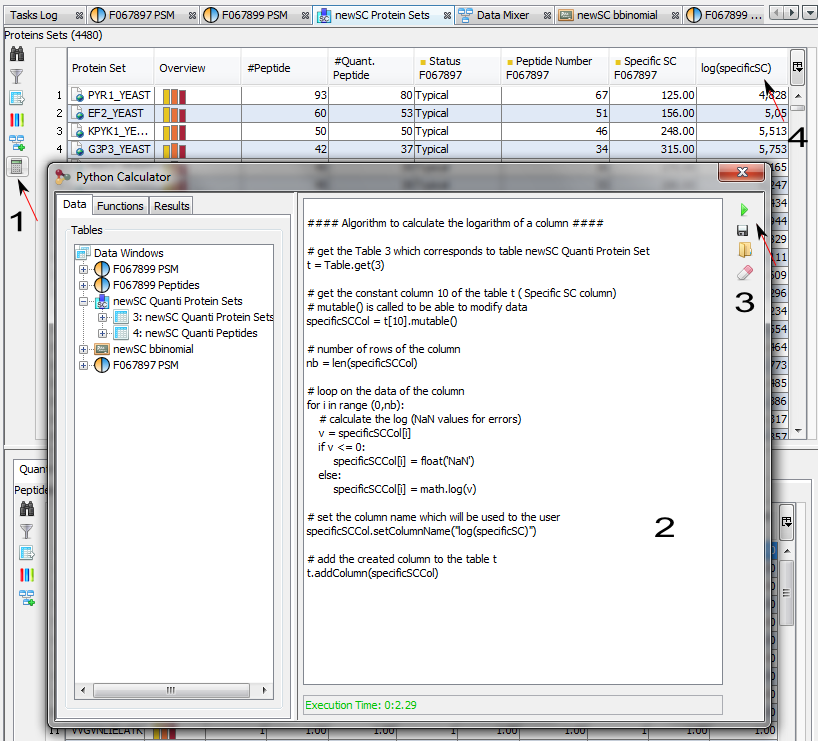
1) To open the calculator, click on the calculator icon (not available on all views for the moment)
On the left part of the calculator, you can access to all viewed data, double click to add a table or a column to the script.
2) Write your python script on the text area
3) Execute it by clicking on the green Arrow.
4) When the script has been executed, the results of the calculations (variables, new columns) are available in the “Results” tab. Double click on a new column to add it to the table. Or like in the example, directly add the column to the table programmatically.
#### Algorithm to calculate the logarithm of a column ####
# get the Table 3 which corresponds to table newSC Quanti Protein Set
t = Table.get(3)
# get the constant column 10 of the table t ( Specific SC column)
# mutable() is called to be able to modify data
specificSCCol = t[10].mutable()
# number of rows of the column
nb = len(specificSCCol)
# loop on the data of the column
for i in range (0,nb):
# calculate the log (NaN values for errors)
v = specificSCCol[i]
if v <= 0:
specificSCCol[i] = float('NaN')
else:
specificSCCol[i] = math.log(v)
# set the column name which will be used to the user
specificSCCol.setColumnName("log(specificSC)")
# add the created column to the table t
t.addColumn(specificSCCol)
#### Algorithm to perform a difference and a mean between two columns ####
t = Table.get(9)
colAbundance1 = t[3]
colAbundance2 = t[5]
# difference between two columns
colDiff = colAbundance1-colAbundance2
# set the name of the column
colDiff.setColumnName("diff")
# mean between two columns
colMean = (colAbundance1+colAbundance2)/2
# set the name of the column
colMean.setColumnName("mean")
# add columns to the table
t.addColumn(colDiff)
t.addColumn(colMean)
#### Algorithm to perform a pvalue and a ttd on abundances column of a XIC quantitation ####
t = Table.get(1)
pvalueCol = Stats.pvalue( (t[2], t[3]), (t[4],t[5]) )
ttdCol = Stats.ttd( (t[2], t[3]), (t[4],t[5]) )
pvalueCol.setColumnName("pvalue")
ttdCol.setColumnName("ttd")
t.addColumn(pvalueCol)
t.addColumn(ttdCol)
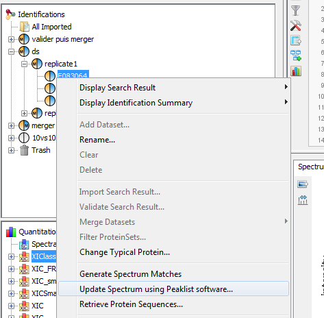
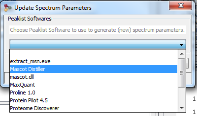
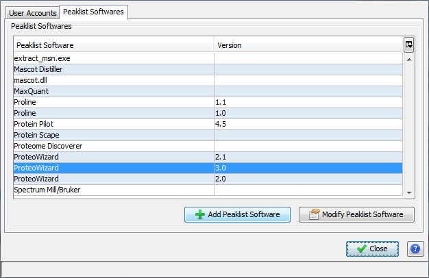
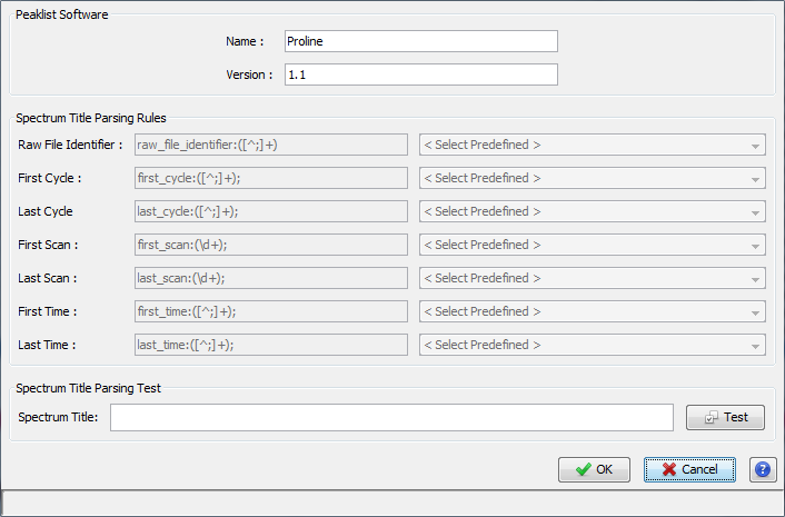
When importing search result, the software used for the peaklist creation has to be specified. This parameter is mandatory for the XIC quantitation as it is used to find scan number or RT in the spectrum title. Indeed, this information is then used to extract abundances in the raw files.
If an invalid software has been specified when importing, it is possible to change the peaklist software afterwards. This option is only valid for Identification DataSets.
Right click on the identification DataSet, and select “Update Spectrum using Peaklist software”
The following dialog will be displayed allowing user to select the peaklist software to used.
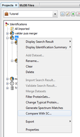
See description of Compare Identification Summaries with Spectral Count.
To obtain a spectral count, right click on a Dataset with merged Identification Summaries and select the “Compare with SC” menu in the popup. This Dataset is used as the reference Dataset and Protein Set list as well as specifics peptides are defined there.
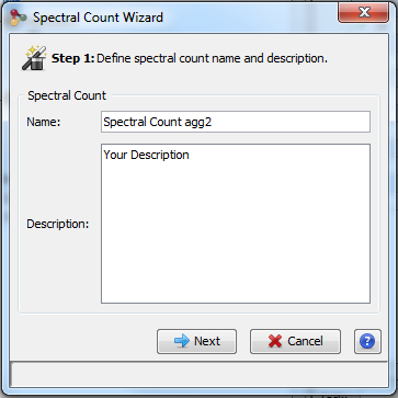
In the Spectral Count window, fill the name and description of your Spectral Count and press Next.
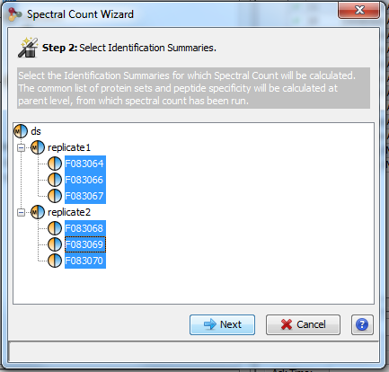
Then select the Identification Summaries on which you want to perform the Spectral Count and press Next.
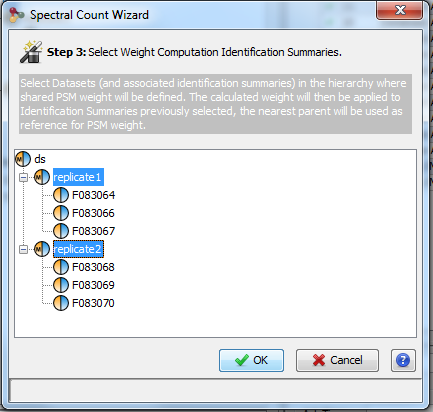
Finally select the DataSet where shared peptides spectral count weight should be calculated and press OK.
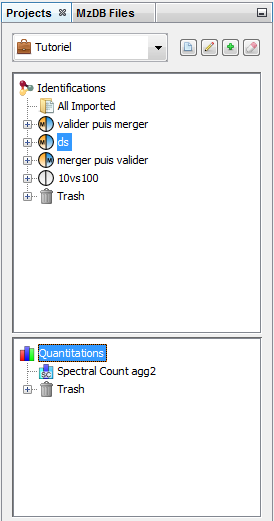
A Spectral Count is created and added to the Quantitations Panel.
You can then display a Spectral Count, see Display a Spectral Count
For description on LC-MS Quantitation you can first read the principles in this page: Quantitation: principles
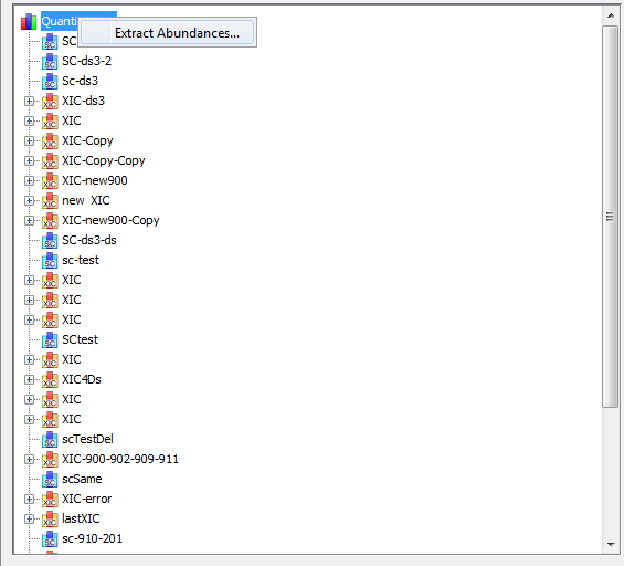
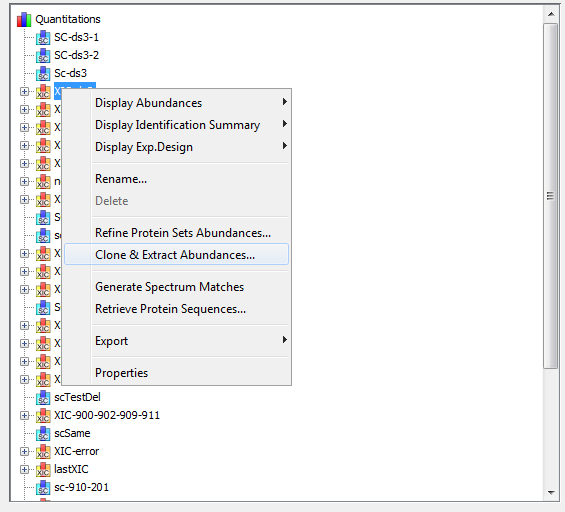
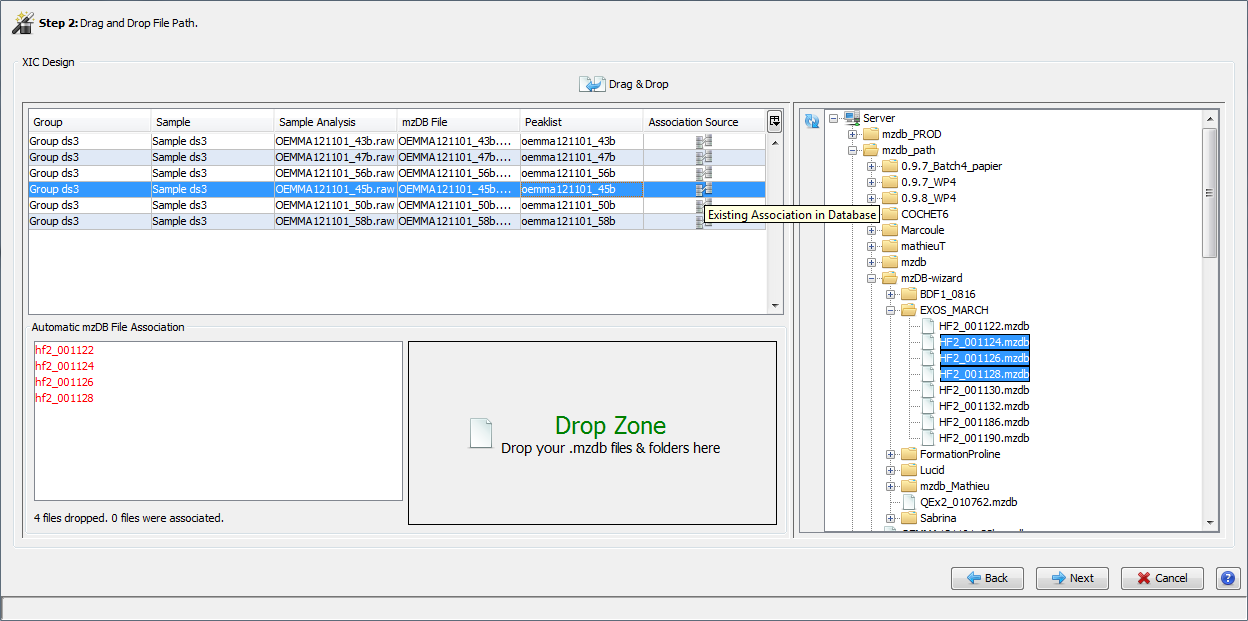
There are two ways to generate a XIC, either by clicking on the “Extract Abundances” action or by selecting the “Clone & Extract Abundances” option, both being located on the respective pop-up menu as shown in the following screenshots. The difference among the two approaches lies on the fact that in the second case, the new XIC is generated for an existing Experimental Design.
To create the Design of your XIC, drag and drop the desired identifications from the right panel to the left one. If you drop an identification on the XIC Node, Group and Sample parents' nodes will be automatically created. You can also directly drop on a Group or Sample Node. Regarding the name of the aforementioned parent nodes, the general rule that is followed dictates that if possible, a parent node name should be based on the children nodes’ earliest common ancestor, if one should exist. Furthermore, since Proline Studio 1.5, the user can further enhance his XiC Design by creating his own Samples and Groups which in turn can populate by dragging inside them elements from the identifications tree. Once more, going to the next step requires that no empty Group and Sample nodes exist within the design.
Furthermore the user has the capacity to rename any node he wishes using a pop-up menu as shown in the screenshot below. Additionally, for Group, Sample or root nodes, renaming can be triggered either by pressing F2 while having the in-question node selected, or by consequently clicking three times on the aforementioned node. Using triple-click somes times can be a little confusing for the user as it can also lead to possible expansion/retraction in the case of a parent node. Finally, it is recommended that at least the XIC node is renamed.
In order to be able to perform any XiC design, all participating Sample Analysis nodes must be associated with a corresponding raw file. If this is not the case, corrective actions must be taken by the users in order to establish those associations. The association can be created at the second step of the XIC design using two different interface features. The first way to establish such a “connection” is by explicitly drag n drop an .mzdb file that is stored on the server file system. It must be noted that although it is possible to overwrite an existing association, the is no mechanism responsible for ensuring compatibility. So it is thus advised, either to avoid such action or to proceed with caution considering the encountered risks.
The second way to establish a missing connection is to use a newly introduced feature in Proline Studio, the Drop Zone. The latter one can be quite handy in cases where multiple associations are missing or when the plethora of uploaded .mzdb files intimidates the user from manually searching the files one by one. The feature itself is extremely easy to use as it just requires dragging a set of files or folders containing .mzdb files from the user part. As soon as a drop takes place, all missing connections will be automatically created as long as a matching .mzdb file has been dropped in the Drop zone. It must also be noted that since version 1.5, users have now at their disposal indices about the association source. Furthermore, in order to protect existing in database association from possible a possible corruption, the latter ones cannot be overwritten.
When the XIC Design is finished, click on the next button and select the parameters. See Label-free LC-MS quantitation configuration to have more details about the different parameters.
The XIC parameters are not all displayed. You can display a complete set of parameters by clicking on the “Advances Parameters”.
Note: all the parameters are already set with default values.
Newly generated XIC designs are immediately added to the Quantitation Tree. Through the latter one, and via a popup menu, the end user has the capacity either to view a design’s properties as seen to the following screenshot, or to apply a series of actions on it, including among others:
Right click on the selected XIC node in the Quantitation tree, and select “Refine Proteins Sets Abundances…”
In the dialog, you can:
- specify peptides to consider for quantitation
- configure parameters used for peptides quantitation
- configure parameters used for proteins quantitation
For more details, see Post-processing of LC-MS quantitative results
You can see the results by displaying the XIC (Display a XIC) or export them Export Data
Since version 1.4 Proline Studio includes a general settings dialog which can be accessed from the top menu bar clicking on “General Settings” as shown in the screenshot below.
The latter one consists of a constantly but slowly growing number of user preferences regarding various aspects of the utilization of Proline Studio. Based on their context, for the time being, preferences are organized into the following four tabs:
JMS Settings tab contains parameters that concern the exchange of messages between your local machine and the JMS Server. It should be made clear that compared to other preferences, preferences that are included in this tab should be treated with caution. Mistreating a communication preference can lead either to communication/connection problems or to users’ confusion to whether they are connected to the correct server version.
Parameter can be seen as a name which represents a server address. The parameter’s existence is justified by the fact that multiple server versions might run on the same server machine imposing the need to be able to canalize Studio’s messages appropriately.
Table parameters’ tab encapsulates a short list of preferences regarding all tables generated throughout Proline Studio. More specifically those preferences control the arrangement of the participating columns as well as their respective width.
This field dictates the spatial arrangement of table columns. Three arrangements are possible:
When “Automatic Columns Size” is used, all columns are width-wise readjusted in a way that they all fit to their container. Given that it is a “fit-to-screen” approach, it lacks scrollbars and does not guarantee the readability of the presented date, especially when the number of columns is high.
On the other hand a simpler approach that guarantees readability is to select “Fixed Column Size”. In this case all table columns have a fixed width, explicitly dictated by the user using the parameter “Column Width”.
The less clear option is “Smart Column Size” which serves as a trade off between the aforementioned ones. It tackles with the cases that either we have too many columns to visualize using the “Automatic” approach or too few and the selected default and globally applied width imposes unneeded scrollbars ending in hiding some columns at the same time. In this context, “Smart Column Size” can be seen as a simple rule based on the ratio between the mean column width needed in case of “Automatic Column Size” for a specific table and the globally selected width. For the sake of simplicity we have set a threshold of 0.7 or 70% which on its turn determines which one of the two first modes will be used given a table. If the ratio is smaller than 0.7 then the table in question will be presented in “Fixed Column Size” mode. On contraire if ratio is equal or greater than 0.7, then we consider that using “Automatic Column Size” mode is more appropriate as it balances between a possible slightly smaller than desired width and the possibility of hiding a column using scrollbars.
The second preference is more or less self explanatory and corresponds to the globally desired columns’ width when fixed rune is applied, either directly or as a result of the smart mode.
In this tab we can find a diverse set of preferences regarding various tasks encountered in Proline Studio. For the time being those preferences are:
Unlike the last three, Hide Getting Started Dialog is pretty much self explanatory. The second preference on the other hand, “Default Search Name Source” affects the way identification datasets are named on importation. For this preference we have three possible options:
This parameter affects the .xls and .xlsx files that are produced in the process of export (client side). It could be easily described as a preservation of any existing Rich Text Feature in a table. (Colors, Font Weight etc.)
Corresponds to the default raw2mzDB converter. While it is left at the discretion of the user, which version to choose, it must be noted that different versions do tend to work better with specific type raw files. Said that, it is also important to understand that in order for a conversion to be successful within Proline Studio, all system requirements set by the specific raw2mzDB version must be met.
Compared to the previous versions, 1.5 of Proline Studio has been enhanced with basic administration functionality. At this moment, this basic infrastructure permits an advanced user, who at the same time holds the status of Admin, to carry a limited range of tasks on accounts and registered in the system Peaklist softwares.
As we can see, regarding user accounts, the respective administration dialog offers us two possibilities, adding a new user account or modifying an existing one. At this time, both actions are quite simplistic, relying on minimalistic popup dialogs as seen in the following two screenshots.
As we can see, both actions share the same interface with the exception of the predefined and not editable login field in the case of user account modification. Finally, it is important to note that at Studio’s Installation, a default admin user is created permitting us to create the rest of the users.
As seen in the preceding screenshot, the Peaklist Softwares tab follows a similar approach with the accounts one. Again, tab permits us to either add one or modify an existing element via popup dialogs triggered by the two respective buttons. In order to add a new Peaklist Software it suffices to click on the button with the homonym reading, action which will trigger the appropriate dialog.
Similarly, as seen in the proceeding screenshot clicking on the modifying button permits the end user to alter a small attributes subset of an existing Peaklist Software.
Proline Web
Prerequisite: You must have an account to login to the server. Ask your administrator to create one if you don't have any. After the installation, the default account is “admin” with password “proline”
- Open your Google Chrome web browser and connect to the address of the server (ask your administrator)
- Enter your username and password and click “OK”.
- To create a project, please follow the instructions detailed on this page.
In order to create and run Quantitation analyses, you must register your MzDB files into Proline databases. To do so, click on the “Settings” button in the bottom bar of the Dataset Explorer application, and go to the “Raw File Registerer” tab.
Note that this operation will override information if some of the files is already registered.
Close the Settings Window.
Open the DataSet Explorer app from the left panel (if closed, open it by clicking on the “apps” button in the upper-left corner of the page)
When the DataSet Explorer is opened, you can see your Project Tree on the left.
To create a New Project, just click on the New project button at the bottom of this panel or in the context menu of the user node.
You must be logged in as an administrator. Click the gear-shaped button in the top task-bar (circled in blue on the right) to open the administrator settings menu.
On the first tab, “User Administration”, you can create a new user by setting up its name, its password, and define whether or not the user will have the “administration” permissions (including applications, users and service management).
Submit the form to create the user. You can manage existing users from the “users” tab.
Please note that the Proline Web Desktop has its own database and its own users collection. However, if you configured the Proline Service running inside the Proline Web Desktop, it will synchronise the Proline Web Desktop and the Proline Core users each time a user logs in the Proline Web Desktop:
The first thing to do in your brand new project is to import Result Files.
There are many ways to open the dedicated tab:
A new tab will open and display the following panel.
Click on Select result files to browse and select them. The left side of the browsing window is meant for the directories. When you click on one of them, its content is shown on the main panel. Choose one or multiple files then click Ok.
Then configure the following parameters:
Master_protein_score * (1-subset threshold)
won't be imported.
Acetyl peptide N-term=H(-6) C(-7) O(-1)
You can now click on “Start Import” to launch the check and the import tasks.
The server checks your files first, then the import itself is launched automatically.
You can follow the current state of your tasks by clicking on the Tasks button at the bottom of the Project Tree panel.
It opens the Tasks Panel, listing all the tasks that have been run in Proline.
When a task is done, you are notified by a small message in the top of the screen, and you can see its status in the tasks window:
All the Result Files you have imported are listed in the Imported Search Results panel you can access by double-clicking the Imported Search Results node in your project tree.
Double click on the Imported Search Results node to open the corresponding grid.
The grid itself allows to:
The grid toolbar allows to:
From the Search Results grid, click on Edit sample names in batch to open the edition window.
In this window, you can copy and paste a grid from, let’s say, an Excel file. Each row corresponds to a result file. It must contain 2 columns: the sample name and either the peaklist file name/raw file identifier/result file name.
Let’s say you have the following grid:
Peaklist File | Condition |
OVEMB150205_21.raw.mgf | UPS1 50 fmol |
OVEMB150205_23.raw.mgf | UPS1 50 fmol |
OVEMB150205_25.raw.mgf | UPS1 50 fmol |
Copy it then paste it into the edition window as shown below. Notice that in this example, we are using the peaklist file name as a reference, so we must specify it in the selectable box on top of the window to update the column name.
You can also double click on a cell to edit its text directly in the edition window.
The result set table will be updated with the new sample names:
As says the warning, if many imported result files share the same raw file identifier, all of them will be impacted by this action.
Once your Result Files have been imported, you can use them to create a new Identification Dataset. To create it from result files, you can:
Note that you can also create an empty dataset to further assemble complex structures using drag and drop in the project tree. However, this way is not favoured.
You should now see a window asking to choose a source of data for your new Dataset.
The only option available yet is Result Set: it allows you to build a new dataset from the Result Files you have imported. Click OK to continue.
In the right panel, two text fields allow you to enter a name and description (optional) for your dataset.
By default, the result sets will be named in the tree using the result file name. You can change that with the Name child results using box. The possibilities are: peaklist file name, raw file identifier, result file name, sample, search title.
To add one or many files to your selection, select them in the grid (you can use the Ctrl and the Shift keys to make a multiple selection), then click on Add to dataset (top-right of the panel). You can also double click on one file to quickly add it to the selection.
To remove any file from the selection, just select them and click on Remove selected Items.
The creation of your identification dataset happens as follows:
Once your Identification Dataset has been created, you can see it on the tree, in the left side of the window. You may need to collapse and expand again the Identifications node to see it appear.
The white icon let you known that it is not yet validated (becomes green when validated).
Double click on the aggregation node to open the identification summary. This panel shows a list of your Identification fractions (corresponding to each imported file) and, after the validation process, it will display the Merged Result Summary infos.
Refer to the previous paragraph to know how to do these steps.
Once you have selected your result files, click on Add annotations. A window shows up, with as many empty lines as selected files.
Let's say you compare 2 conditions, and you have the following result table (Excel file for instance). The idea is to copy/paste this table to the annotation editor.
Result file | Peaklist File | Condition |
F078594.dat | OVEMB150205_21.raw.mgf | UPS1 50 fmol |
F078596.dat | OVEMB150205_23.raw.mgf | UPS1 50 fmol |
F078592.dat | OVEMB150205_25.raw.mgf | UPS1 50 fmol |
F078590.dat | OVEMB150205_27.raw.mgf | UPS1 50 fmol |
F078591.dat | OVEMB150205_12.raw.mgf | UPS1 5 fmol |
F078595.dat | OVEMB150205_14.raw.mgf | UPS1 5 fmol |
F078597.dat | OVEMB150205_16.raw.mgf | UPS1 5 fmol |
F078593.dat | OVEMB150205_18.raw.mgf | UPS1 5 fmol |
Click OK to register these annotations. The window closes and the files selection has been annotated as shown below (on the left). Click Create Dataset. The generated dataset (below, on the right) has 2 levels of aggregation: biological group (with the copy/pasted names) and top-level (chosen name for dataset).
Let's take a slightly more complex design, introducing biological replicates for each condition:
Result file | Peaklist File | Biological replicate | Condition |
F078594.dat | OVEMB150205_21.raw.mgf | BRep 1 | UPS1 50 fmol |
F078596.dat | OVEMB150205_23.raw.mgf | BRep 1 | UPS1 50 fmol |
F078592.dat | OVEMB150205_25.raw.mgf | BRep 2 | UPS1 50 fmol |
F078590.dat | OVEMB150205_27.raw.mgf | BRep 2 | UPS1 50 fmol |
F078591.dat | OVEMB150205_12.raw.mgf | BRep 1 | UPS1 5 fmol |
F078595.dat | OVEMB150205_14.raw.mgf | BRep 1 | UPS1 5 fmol |
F078597.dat | OVEMB150205_16.raw.mgf | BRep 2 | UPS1 5 fmol |
F078593.dat | OVEMB150205_18.raw.mgf | BRep 2 | UPS1 5 fmol |
Note In most of the cases, the definitions go as following:
- biological group = biological condition
- biological sample = biological replicate
- sample analysis = technical replicate
However, these definitions are not strict and you can use and adapt the hierarchy to fit your needs.
Click OK to register the annotations and see them in the creation panel.
Then click Create Dataset.
The generated dataset has 3 levels of aggregation:
To launch a validation on a dataset:
The following form appears:
The validation form handles several settings, especially:
When ready, click on Validate to launch the validation task. You can see it in the tasks panel. When the validation finishes, a notification is displayed and the node icon is colored in green.
See more details about the validation process.
You can either create a quantitation from scratch, meaning you enter all information; or clone an existing quantitation to pre-fill the form with previous parameters.
Right-click on a quantitation, then on Clone (new quantitation).
This will open the quantitation launcher, with pre-filled parameters.
The new quantitation name will be, by default, the same as the cloned quantitation, suffixed by “(copy)”. You can change it.
When cloning, a popup window will appear, offering to Use the previous peakels detections. This mean the software will not look for signal again, but use the peaks that were found in the first quantitation. This will dramatically reduce the computation time.
You can change this parameter afterwards in the LFQ parameters section of the form (see description below).
There are 2 ways to open the Quantitation Creation form:
The first tab of the creation panel, entitled Information, let you define a name and an optional description for your quantitation. Type and method are disabled since the label free base on abundance extraction is the only combination available yet.
Click on Next to go to the next step.
The Experimental design tab is where you define your Groups and Samples.
The simplest way to create biological groups (e.g. representing biological conditions) is to drag the validated nodes from the project tree and drop them in the dedicated zone. Drag/drop the nodes one by one.
In the example below, two groups are created this way:
For more complex experimental design, click on Add New Sample to add a sample (e.g. biological replicate) to your group. Enter the name of the sample, then drag/drop the corresponding node to the right panel to add it.
In most of the cases, the definitions go as following:
However, these definitions are not strict and you can use and adapt the hierarchy to fit your needs. Tooltips are available to help you remind it (place your mouse over the terms to see them).
Once you have prepared all your groups and samples, click on the Next button.
This tab let you set up you abundance extraction parameters.
Depending on your choices, some parameters will become available/unavailable (e.g. clustering parameters are visible only when extracting from MS/MS events).
Tooltips are available to help you understand each parameter (keep he mouse on a parameter name to see it appear).
See more details on these parameters.
See more details on the quantitation process.
Tip: If you are creating a quantitation that you have already done in the past (i.e. using the same files), select the Use previous peakel detection to go much faster. It will skip the long step of peakel detection and use what was previously found instead.
Click on Next to go to the last tab.
The purpose of this tab is to define the ratios between the groups your quantitation will rely on.
You can define the ratios:
Click the “double arrow” icon to invert numerator and denominator in a ratio.
When you're done, just press the Launch Quantitation button. You will be noticed when the task is finished
You can delete an Identification dataset by:
All deleted datasets are visible in the Trash node in the project tree.
Double-click on an identification or an aggregation of identifications to open its summary and results panel.
The Summary panel sums up the validation parameters and results.
If you clicked on an Aggregate node, this panel shows the information of the Merged Result Summary and a grid listing all of the identifications of this aggregate.
If you clicked on a result set (a leaf in the tree, corresponding to a single file), then the Summary panel will display its validation parameters; including the parameters chosen when launching the validation and the ones that were automatically computed.
In order to browse the protein set data of a validated identification, click on the validated identification node in the project tree, on the left side panel of the dataset explorer, and then open the Proteins tab.
IMPORTANT: Please note that the Protein Table only displays the validated proteins. Furthermore, they actually are the representative math of a protein set.
Note that the identified proteins can be marked as Favorite. See the dedicated documentation here.
When clicking a protein, the other tables will be filled with related information:
Each table of the Identification data viewer provides a set of Filters for numerical, text and boolean data. It is placed on the left of the grid. They are circled in red in the first screenshot. Click on the double arrow to fold/unfold these panels. Use them as follows:
The Peptides tab of a validated Identification Dataset (or Merged Dataset) allows you to browse the peptides of the related Result Summary.
Note that the identified peptides can be marked as Favorite. See the dedicated documentation here.
When clicking a peptides, the Peptide Matches and Protein Matches tables are filled with entities related to this peptide. Double-click on one of these entities to open the dedicated tab and focus on it.
Each table of the Result Summary data viewer provides a set of Filters for Numerical, Text and Boolean data, placed on the left of the grid.
The MS Queries table displays the MS Queries of the Result Summary and offers the same filters options as the others tables.
Double-click on a quantitation node in the Project Tree in order to open its tabbed-panel.
There are 3 tabs under the Summary: Experimental design, LFQ Params and Stats Params.
It also provides the “Post processing” tool you need to launch in order to compute statistics on your data (get ratios information). Note that the quantified proteins and peptides tables must be reloaded after the post processing (use the Refresh icon on the table top right).
This panel is a summary of your experimental design, listing your biological groups, their samples and their technical replicates.
It has exactly the same layout as the quantitation launcher form, but is not editable. It allows you to see with which parameters the label-free quantitation was run.
It has exactly the same layout as the parametrization window for the post processing, but is not editable. It allows you to see the parameters used for the last post processing of the quantitation.
This tab won’t be shown if no post processing has been run on this quantitation.
The graphics are related to the files (quantitation channels) in which the protein has been -or not- quantified. Tooltips are available by keeping the mouse over a bar or a dot of the graphics.
The quantified proteins can be marked as Favorite. See the dedicated documentation here.
As for the identification, the tables Protein Set Matches and Master Quant. Peptide will be filled when a protein is clicked.
This grid is also provided a filter tool that you can use as follows:
Double-clicking a Protein will open the Protein details panel:
On this panel, you get an insight of all quantified peptides for this protein (double click on the peptide in the 'Quantified Peptides' table or expand directly the peptide panel).
You can click on the eye icon (circled in green) to access the Speclight viewer of this Peptide.
TODO: insert link to Speclight doc
This is the list of all quantified peptides.
The quantified peptides can be marked as Favorite. See the dedicated documentation here.
Note that the peptide grid has got a filter tool too.
This panel offers two tabs to give you information about the LC-Ms maps of the experiment.
IMPORTANT: it is crucial to visit this graphics to manually control the processed map alignments. A bad alignment (showing many curve trends, or too large time deltas) will lead to quantitation errors. If you have the feeling that the alignment needs improvement, re-run the quantitation, tuning the Alignment Computation part of the LFQ Params tab (see how to create a quantitation).
On this chart, you can see all the delta time of each LC-MS map against the reference LC-MS map. The reference map is the one specified in the title of the chart. It corresponds to the x axis.
Click on one or many raw files to display their LC-Ms map features.
This panel lists all the features detected and processed by Proline.
Click a master feature to see: - the corresponding XIC on the right-side panel - the corresponding features in each file in the bottom grid (first tab) - the corresponding master quant. peptide ion in the bottom gris (second tab).
You can double click an entry in the bottom grid to open a dedicated tab (feature/peptide ion details).
All the peaks are listed here, independently from the features they have been gathered to.
In order to see the statistics on the ratios, you have to launch the Post Processing (previously called Profile Analysis). Launch it from the Summary tab toolbar, or from the quantitation node (in project tree) context menu.
You can see the Post Processing configuration window below.
See more details on the post-processing parameters.
Launch the post processing by clicking Run. You can watch the task progression in the Tasks window. You will also be notified when the task is done. You can then watch the results in the Quantitation Stats tab.
This tab offers many panel to help you visualize statistics about your quantitation.
The first panel is a volcano chart of your Proteins based on their -Log10 T-Test P-Value over Log2 Ratio.
The Left grid shows a list of all the proteins, and if they are in the actual boundaries of the selection/exclusion tool.
Hover a dot to see information on the protein.
Click on it to open its protein details panel.
The AC Filters let you select a color (by clicking on it) and enter an Accession Number (or a part of it) to highlight matching proteins on the chart). In this example, all proteins containing “HUMAN” in their accession number are colored in orange. By defaults, dots are light blue.
The Log2 Fold Change (of the ratios) and P-Value fields let you define new boundaries for the protein selection/exclusion. It is shown on the chart with black lines and gray points to show excluded proteins.
Select a zone with the mouse cursor to zoom on it. Use the icon at the top-right of the volcano plot to export it at several picture formats.
The second tab offers the same volcano chart and options for peptides. Instead of accession number, you can color the dots according to their sequence or PTM definition.
In the tree, you can organize your quantitations into folders. To create a new folder, right click on the Quantitations node, then on Create folder. Enter a name for the folder. You can now drag and drop quantitations or other folders into the newly created one. You can also drag and drop quantitations/folders out of a folder.
Four kind of entities can be labeled as “favorite”: the identified proteins, the identified peptides, the quantified proteins and the quantified peptides.
The column entitled Favorite in each table corresponding to those entities allows to:
There a 3 levels of favorites:
Click on the star icon of the protein or peptide you want to update. A contextual menu will open, with 3 options:
You can set as favorite any entity that is not yet marked so (blue and grey stars).
Unsetting an entity as favorite will apply this change only in the current dataset (if it was labeled as favorite in another dataset, the latter won’t be affected).
You can also use the Favorites menu of the grid to set/unset all the grid items as favorites. You may want to filter the grid before.
In the example above, all proteins that were quantified in at least 7 files and have a protein set score superior to 150 will be set/unset as favorites in one click.
Since the favorite status of an entity is coded with an integer, you can sort the Favorite column (use the header menu) and/or filter the grid items on their “favorite status”. To do so, use the Button Data tab of the filter.
When you marked an entity as favorite, you may want to know if it was also set as favorite in other datasets.
To do so, click on the star icon the select See references in project.
The panel below will open.
In this panel, you will see every reference of the entity that has been marked as a favorite. You can click a green arrow to open the corresponding panel, focused on the entity.
All grids are copyable, but not all the same way.
The grids with a “Save” icon on the top right can be copied entirely (the whole content) with this icon.
The others can be copied line by line (select several lines by maintaining Shift actioned while clicking on the lines, or select all lines with Ctrl+A) with the keys Ctrl+C.
The “Export” button of any identification or quantitation node is accessible by right-click on it, or in its summary tab when you double-click on it. All your exported data will appear under the “Exported Files” node of the project you chose during export (the dataset current project, by default).