Proline User Guide
Release 2.1
Proline is a production grade software suite, which provides an environment for large-scale MS data management, visualization, analysis and curation with the main objective of promoting the production and sharing of high quality proteomic datasets. Proline can be used (i) to produce reliable identification and quantification results through robust automated processes, (ii) for data curation, (iii) to systematically save and keep track of metadata from processing steps, parameters and generated data, and (iv) to submit highly qualified datasets to public repositories.
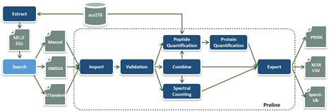
A workflow in Proline is implemented as a collection of tasks (see Figure) that can be performed by the user through the graphical user interface. Users can import multiple identification results corresponding, for example, to fractions and replicates of a biological sample and combine them before or after validation. The resulting datasets can then be compared or quantified using spectral counting or DDA label-free quantification, before exporting the results in different file formats.
The software suite is based on two main components: a server handling processing tasks and based on relational database management system storing the data generated and two different graphical user interfaces, both allowing users to start tasks and visualize the data: Proline Studio which is a rich client interface and Proline Web the web client interface. An additional component called ProlineAdmin is used by system administrators to set up and manage Proline. Proline Zero is an all-in-one, “zero installation” solution containing the server and Proline Studio.
This document is organized in two sections:
Proline Concepts & Principles
Proline considers different types of identification data: Result Files, Search Results and Identification Summaries which will be defined in the following sections.
A result file produced by a search engine can be imported into Proline in their native format. OMSSA (.omx files), Mascot (.dat files) and X!Tandem (.xml files) search engines are currently supported. In addition, the mzIdentML format is supported to allow the output from any other search engine compatible with this standard to be imported (e.g. MS-GF+). A first version for MaxQuant support has been implemented. It is possible to import only search results or to import search results as well as quantitation (beta version) values from MaxQuant files.
Search engines may provide different types of searches for MS and MS/MS data. It is important to highlight that Proline only supports MS/MS ions searches at this point.
A search result is the raw interpretation of a given set of MS/MS spectra given by a search engine. It contains one or many peptides matching the submitted MS/MS spectra (PSM, i.e. Peptide Spectrum Match), and the protein sequences these peptides belong to. The search result also contains additional information such as search parameters, used protein sequence databank, etc.
A search result is created when a result file is imported in Proline. During this step, no filtering or thresholding is applied: along with the search parameters, all submitted spectra, peptide spectrum matches (PSMs) and protein hits suggested by the search engine are retained in the Proline database to allow subsequent validation of putative identifications. In the case of a target-decoy search, two search results are created: one for the target PSMs, one for decoy PSMs.
Importing a result file creates a new search result in the database which contains the following information:
Proline handles decoy searches performed from two different strategies:
An Identification Summary is a set of identified proteins inferred from a subset of the PSM contained in the search result that have been declared valid. The subset of PSM taken into account are the PSM that have been validated by a filtering process (example: PSM fulfilling some specified criteria such as score greater than a threshold value).
All peptides identifying a protein are grouped in a Peptides Set. A same Peptides Set can identify many proteins, represented by one Proteins Set. In this case, one protein of this Protein Set is chosen to represent the set, it is the Typical Protein. If only a subset of peptides identify a (or some) protein(s), a new Peptide Set is created. This Peptide Set is a subset of the first one, and identified Proteins are Subset Proteins.
All peptides sets and associated protein sets are represented, even if there are no specific peptides. In both cases above, no choice is done on which protein set / peptide set to keep. These protein sets could be filtered after inference (see Protein sets filtering).
There are multiple algorithms that could be used to calculate the Proteins and Protein Sets scores. Proteins scores are computed during the importation phase while Protein Sets scores are computed during the validation phase.
Each individual protein match is scored according to all peptide matches associated with this protein, independently of any validation of these peptide matches. The sum of the peptide matches scores is used as protein score (called standard scoring for Mascot result files).
Each individual protein set is scored according to the validated peptide matches belonging to this protein set (see inference).
The score associated with each identified protein (or protein set) is the sum of the score of all peptide matches identifying this protein (or protein set). In case of duplicate peptide matches (peptide matched by multiple queries) only the match with the best score is considered.
This scoring scheme is also based on the sum of all non-duplicate peptide matches score. However the score for each peptide match is not its absolute value, but the amount that it is above the threshold: the score offset. Therefore, peptide matches with a score below the threshold do not contribute to the protein score. Finally, the average of the thresholds used is added to the score. For each peptide match, the “threshold” is the homology threshold if it exists, otherwise it is the identity threshold. The algorithm below illustrates the MudPIT score computation procedure:
Protein score = 0
For each peptide match {
If there is a homology threshold and ions score > homology threshold {
Protein score += peptide score - homology threshold
} else if ions score > identity threshold {
Protein score += peptide score - identity threshold
}
}
Protein score += 1 * average of all the subtracted thresholds
The benefit of the MudPIT score over the standard score is that it removes many of the junk protein sets, which have a high standard score but no high scoring peptide matches. Indeed, protein sets with a large number of weak peptide matches do not have a good MudPIT score.
This scoring scheme, introduced by Proline, is a modified version of the Mascot MudPIT one. The difference with the latter is that it does not take into account the average of the substracted thresholds:
Protein score = 0
For each peptide match {
If there is a homology threshold and ions score > homology threshold {
Protein score += peptide score - homology threshold
} else if ions score > identity threshold {
Protein score += peptide score - identity threshold
}
}
This score has the same benefits than the MudPIT one. The main difference is that the minimum value of this modified version will be always close to zero while the genuine MudPIT score defines a minimum value which is not constant between the datasets and the proteins (i.e. the average of all the subtracted thresholds).
Once a result file has been imported and a search result created, the validation is performed in four main steps:
Finally, the identification summary issued from these steps is stored in the identification database. Different validation of a Search Result can be performed and a new Identification Summary of this Search Result is created for each validation.
When validating a merged Search Result, it is possible to propagate the same validation parameters to all childs Search Results. In this case Peptide Matches filtering and validation will be applied on childs as well as Protein Sets filtering. Note: actually, Protein Sets validation is not propagated to childs Search Results.
Peptide Matches identified in search results can be filtered using one or multiple predefined filters (described hereafter). Only validated peptide matches will be considered for further steps.
All PSMs with a score lower than a given threshold are discarded. For some search engines, Proline computes the PSM score value itself by applying a mathematical transformation to another PSM property. For instance, the score values for PSMs from X!Tandem search results correspond to the log10 transformation of the PSMs expectation values.
This filter is applied after having temporarily joined target and decoy PSMs corresponding to the same query. For each query, target/decoy PSMs are then sorted by score. As in Mascot, a pretty rank is computed for each PSM depending on their ranking: PSM with almost equal score (difference < 0.1) are assigned the same rank. All PSMs with a pretty rank greater than the cut-off specified are discarded.
PSMs corresponding to peptide sequences shorter than the cut-off stipulated will be discarded when this parameter is applied.
This filter is used to select PSMs based on the Mascot expectation value (e-value) which reflects the difference between the PSM’s score and the Mascot identity threshold (p=0.05). PSMs with an e-value greater than the threshold specified are discarded.
Proline can compute an adjusted e-value. It first selects the lowest threshold between the identity and homology e-values (p=0.05). Then, it computes the e-value using this selected threshold. PSMs for which the adjusted e-value is greater than the specified cut-off are discarded.
Given a specific p-value, the Mascot identity threshold is calculated for each query and all peptide matches associated with the query for which the score is lower than the identity threshold calculated are discarded.
Given a specific p-value, the Mascot homology threshold is inferred for each query and all peptide matches associated with the query which have a score lower than the calculated homology threshold are discarded.
This filter validates only one PSM per Query. To select a PSM, following rules are applied:
For each query:
For testing purposes, it is possible to request for this filter to be executed after Peptide Matches Validation (see below). In this case, the requested FDR in validation step is modified by this filter. This is just to confirm the need or not of this filter and to validate the way we apply it!
This filter selects only one PSM per pretty rank, which is already the case when a given pretty rank is associated with a single PSM. When multiple PSMs have the same pretty rank, Proline will retain the peptide associated with the protein that has the highest number of MS/MS events.
Thus, if this filter is combined with the “Pretty rank” filter, the result obtained should be identical to the result of the “Single PSM per MS query” filter.
For testing purposes, it is possible to request for this filter to be executed after peptide matches validation . In this case, the requested FDR in validation step is modified by this filter. This is just to confirm the need or not of this filter and to validate the way we apply it!
In addition to these filters, a target-decoy validation approach (Elias and Gygi, 2007) can be performed at PSM level by adjusting a user-specified validation criterion until it reaches a user-specified false discovery rate (FDR). The search engine score can be used as a generic validation criterion for any of the search engines supported by Proline. For results obtained with the Mascot search engine, other criteria can be used to control the FDR: Mascot e-Value, Mascot adjusted e-Value, Mascot p-Value based on identity threshold, or Mascot p-Value based on homology threshold.
There are several ways to calculate FDR depending on the database search type. In Proline the FDR is calculated at PSM and protein levels using the following rules:

Note: when computing PSM FDR, peptide sequences matching a Target Protein and a Decoy Protein are taken into account in both cases.

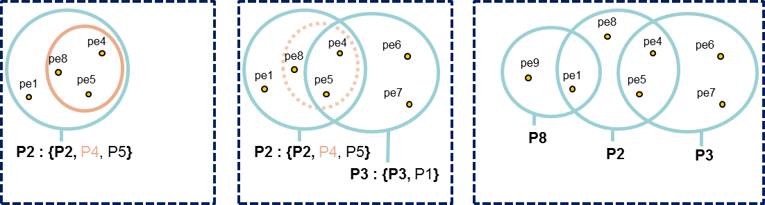
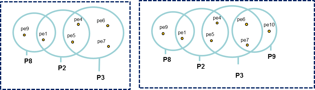
Any Identification Summary, generated by a validation process or by merging datasets could be filtered.
Filtering consists in invalidating Protein Sets which doesn't follow specified criteria. Invalidated Protein Sets are not taken into account for further algorithms or display.
Available filtering criteria are defined below.
This filter invalidates protein sets that don't have at least x peptides identifying only that protein set. The specificity is considered at the DataSet level.
This filtering goes through all Protein Sets from worse score to best score. For each, if the protein set is invalidated, associated peptides properties are updated before going to the next protein set. Peptide property is the number of identified protein sets.
This filter invalidates protein sets that don't have at least x peptides identifying that protein set, independently of the number of protein sets identified by the same peptide.
This filtering goes through all Protein Sets. For each, if the protein set is invalidated, associated peptides properties are updated before going to the next protein set. Peptide property is the number of identified protein sets.
This filter invalidates protein sets that don't have at least x different peptide sequences (independently of PTMs) identifying that protein set.
This filtering goes through all Protein Sets from worse score to best score. For each, if the protein set is invalidated, associated peptides properties are updated before going to the next protein set. Peptide property is the number of identified protein sets.
This filter invalidates protein sets which score is below a given value.
Once prefilters (see above) have been applied, a validation algorithm can be run to control the FDR. See how FDR is calculated.
At the moment, it is only possible to control the FDR by changing the Protein Set Score threshold. Three different protein set scoring functions are available.
Given an expected FDR, the system tries to estimate the best score threshold to reach this FDR. Two validation rules (R1 and R2) corresponding to two different groups of protein sets (see below the detailed procedure) are optimized by the algorithm. Each rule defines the optimum score threshold allowing to obtain the closest FDR to the expected one for the corresponding group of protein sets.
Here is the procedure used for FDR optimization:
The separation of proteins sets in two groups allows to increase the power of discrimination between target and decoy hits. Indeed, the score threshold of the G1 group is often much higher than the G2 one. If we were using a single average threshold, this would reduce the number of G2 validated proteins, leading to a decrease in sensitivity for a same value of FDR.
Identification results can be combined to construct a parent dataset, and create a non-redundant list of identified peptides and proteins. This combination can be performed either before validation (on search results) or after validation (on identification summaries). Since this operation could be recursively performed, it leads to hierarchical structuring of search results and/or identification summaries. On the one hand, combination before validation (taking into account all PSMs identified by the search engine) may, for example, be relevant when analyzing results obtained after peptide fractionation: in that case, several peptides belonging to the same protein may be spread across different result sets; these sets should be merged before protein validation. On the other hand, merging identification summaries is appropriate when seeking to group the validated results from series of individual samples to be compared or when combining data from different search engines.
When datasets are combined, their PSMs are collected to generate a non-redundant set of peptides before recomputing protein inference. Additionally, the mappings between peptides and FASTA entries observed across the different datasets are also collected and merged into a single final mapping list. This list reflects thus the whole set of peptide and protein matches that were observed in the individual datasets.
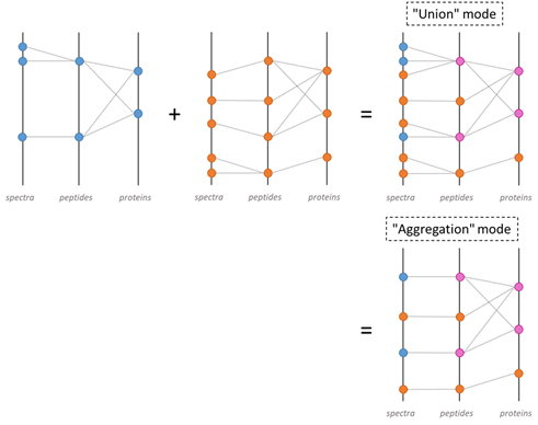
Users can combine search results or identification summaries. The main difference is the set of spectra and peptides (and thus PSMs) considered. When combining search results, all spectra, peptides and PSMs in the dataset are considered, whereas when combining identification summaries, only validated PSMs are taken into account. In addition, Proline can be used to control how PSMs are collected in the parent dataset: in union mode, PSMs originating from combined datasets are added, while in aggregation mode, all PSMs identifying the same peptide are aggregated into a single representative PSM.
Combining datasets in Proline. Datasets are represented as a tripartite graph composed of spectra, peptides and proteins; edges between spectrum and peptides represent PSM. When the blue and orange datasets are combined, PSMs from both datasets are collected together, generating a non-redundant set of peptides. The combination can be performed in 2 modes: union or aggregation mode.
A list of Post translational modification (PTM) sites identified among the peptides of an identification summary can be extracted by Proline. A modification site is characterized by a modification type, at a given location on a given protein. The list of modification sites extracted by the software is restricted to the proteins that are representative of a validated protein set and to the modifications of interest specified by the user. This means that a peptide identified with two different modifications of equal interest to the user will appear twice in the list, one for each modification location.
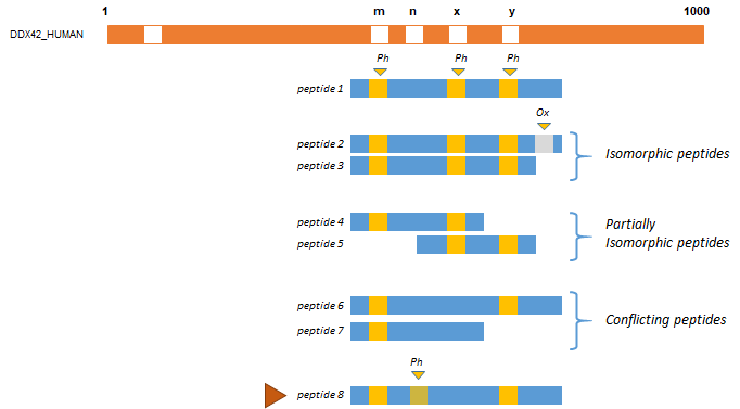
In a second phase, co-localized modification sites are grouped into clusters as soon as an evidence of their co-existence exists. The required evidence is a peptide sequence identified in the dataset with all the clusterized modification sites.
The figure below represents different peptides (blue rectangles), co-localized on a protein sequence (in red). In this example, modifications of interest (Phosphorylation (Ph)) are shown in orange. Peptide 1 proves that Phosphorylation at positions m, x and y occurs simultaneously. Peptides 2 and 3 are considered as isomorphic since the oxidation of peptide 2 is ignored (only Phosphorylations have been declared of interest by the user in this example). Peptides 4 and 5 are partially isomorphic: they confirm Phosphorylation respectively at position (m, x) and (x, y). Conversely peptides 6 and 7 are not in accordance, suggesting that there are two other proteoforms, one with Phosphorylations at position (m,y) but no modification at x and one with a Phosphorylation at position m but not at x. These two peptides could be grouped into another cluster.
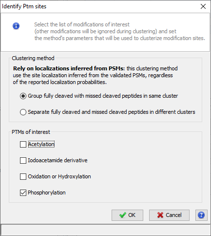
The user can choose between two different different modification clustering methods:
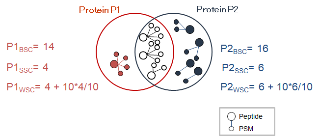
Proline can be used to compare protein sets based on spectral counts through a previously presented algorithm (Hesse et al., 2016). This algorithm notably computes a weighted spectral count metric (called adjusted spectral count in the original publication). Basically, the algorithm takes both unique and shared peptides into account, and for each shared peptide, the proportion of MS/MS spectra that should be attributed to the different protein sets is determined. This proportion (also called weight) is based on the spectral counting of proteotypic (or specific) peptides identifying the different protein sets sharing the peptide to be attributed.
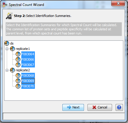
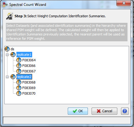
Spectral counting is calculated from a hierarchy of identification summaries. The parent identification summary (at the top of the hierarchy) is where the list of protein sets to compare and the list of specific peptides are created. The list of specific peptides is then used to compute the protein sets respective weights but users can choose any“child” dataset where the weights must be calculated.
First, Proline compute the peptide spectral count at each level of the dataset hierarchy using the following rules:
Once, peptide spectral count is calculated for each peptide, the protein spectral count is computed using the following rules:
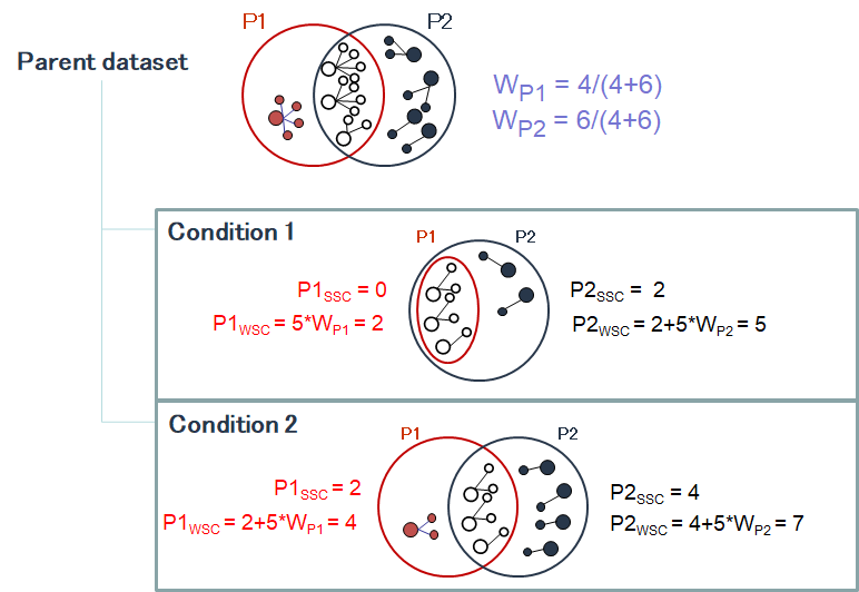
The protein set respective weights computation is based on the proteotypic peptides. The level in the dataset hierarchy where these weights are calculated can be chosen by the user, it could be the top level of the dataset hierarchy or at a lower level. In the following example, the weights (WP1 and WP2) are calculated at the “parent dataset” level. At this level, P1 and P2 are respectively identified by the red and dark blue peptides/psm, each protein set weight is calculated using their specific spectral counting. These weights are thus used to calculate the weighted spectral count of P1 and P2 in the two “child” dataset “Condition 1” and “Condition 2”.
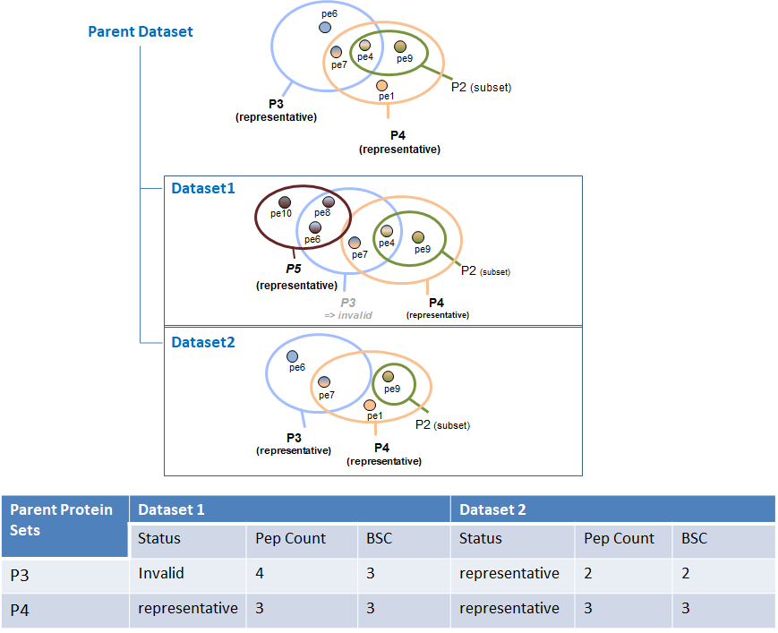
When running SC even on a simple hierarchy (1 parent, 2 childs) in some cases we obtain a BSC value smaller than the peptide count of the protein set. This occurs only for invalid protein sets. Invalid protein sets are the one that are present at the parent level but are filtered at child level (if a specific peptide filter have been applied for example).
Indeed, the peptide count value is read in the child protein sets. On the other hand, the BSC is calculated by getting the spectral count information at child level for each peptide identified at parent level. If a protein set is invalid, its peptides are not taken into account during the merging so some of them could be missing at parent level if they were not identified in the other child.
This case is illustrated in the following figure:
Proline detects chromatographic peaks from raw data converted to the mzDB format (Bouyssié et al., 2015). The converter, named raw2mzdb is based on ProteoWizard, ensuring compatibility with a wide range of instrument vendors.
After a first signal extraction step, the algorithm associates the chromatographic peaks detected with validated PSMs, first by retrieving the corresponding MS/MS spectra acquired during the peptide elution, and then by matching the precursor m/z value of these spectra to the chromatographic peak m/z value. After the deisotoping step, the abundance of each ion is estimated from the apex of the chromatographic peak, which corresponds to the theoretically most abundant isotopologue (inferred from the peptide’s atomic composition). The software then aligns the retention time of these annotated ions for all the LC-MS runs to be compared, and uses this information to cross-assign MS/MS data to ions (i.e. chromatographic peaks) that were detected but not identified in other runs . The resulting ion abundances are finally stored in the Proline database, making them available for rapid data visualization and further post-processing.
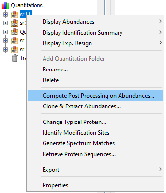
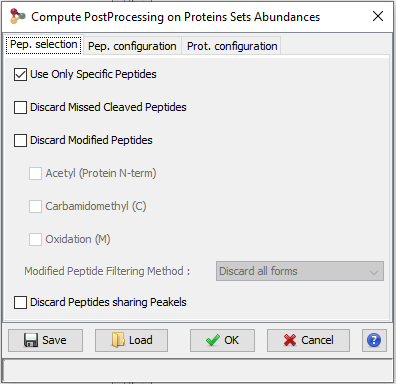
Finally, peptide ion measurements can be summarized as protein abundances using different computational methods. The user can opt to perform additional operations such as excluding peptides or ions based on their characteristics (missed cleavages, variable modifications, sequence specificity, etc.) or normalizing peptide and protein abundances between runs. These post-processing steps can be executed on-demand using different parameters or methods; there is no need to repeat the whole quantification process when changes are made.
During an LC-MS experiment, the m/z and intensity values for each peptide ion detected are recorded in MS1 scans acquired during the elution of this peptide from the chromatographic column. Most existing peak picking algorithms analyze these MS scans individually or sequentially. The Proline algorithm performs the signal detection in a different way. It first takes advantage of the mzDB format to detect chromatographic peaks in spectrum slices (5 m/z wide by default) across the whole chromatographic time. Then, in a given slice, m/z peaks are sorted in decreasing order of intensity. Thus, starting from the most intense m/z peak (apex), the algorithm searches for a peak with the same m/z value in the previous and subsequent MS1 scans, while applying a user-defined m/z tolerance. This lookup procedure stops when the ion signal is absent from more than a predefined number of consecutive scans. The [RT, m/z, intensity] peak list obtained, which is comparable to an extracted ion chromatogram (XIC), is then smoothed using a Savitzky-Golay filter (Savitzky and Golay, 1964). The resulting smoothed chromatogram is then split into the time dimension to form chromatographic peaks, by applying a peak picking procedure that will search for significant minima and maxima of signal intensity. When the signals of two ions overlap in the time dimension, a minimum is generally surrounded by two maxima. If the corresponding valley is deep enough, i.e. at least 66% of the lower surrounding maximum, this minimum will be considered significant (and thus will trigger the generation of two peaks). Once the smoothed chromatogram has been fully analyzed, the algorithm removes the corresponding detected peaks from the current spectrum slice, and performs another lookup using the next available apex. The result of this whole procedure is a list of chromatographic peaks defined by an m/z value, an apex elution time and an elution time range.
These parameters are used by signal extraction algorithms.
In a single run, validated PSMs are MS/MS spectra assigned to a peptide sequence, and each spectrum is characterized by a precursor mass, a charge state and a retention time (RT). The algorithm assigns PSMs to detected chromatographic peaks by matching the spectrum precursor m/z ratio to the chromatographic peak m/z and verifies that the spectrum retention time falls within the peak time range. The PSM charge state assigned is then used to search for chromatographic peaks corresponding to the ion’s isotopologues, considering the precursor mass-to-charge ratio of the spectrum as the monoisotope. The peptide ion intensity is summarized by retaining only the apex of the peak corresponding to the theoretically most abundant isotopologue (inferred from the peptide’s atomic composition). All peptide ion signals (a.k.a. LC-MS features) extracted from an mzDB file and assigned to a PSM are used to construct an LC-MS map. For the sake of simplicity no distinction is made between LC-MS runs and LC-MS maps in this manuscript.
Clustering is applied to group peakels that are matching the same identified ion.
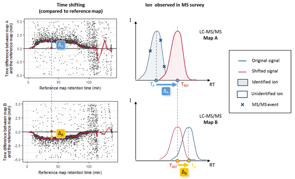
As soon as the PSM are matched to peakels, the software then aligns the retention time of the annotated ions for all the LC-MS runs to be compared, and uses this information to cross-assign MS/MS data to ions (i.e. chromatographic peaks) that were detected but not identified in other runs. Because chromatographic separation is not completely reproducible, LC-MS runs must be aligned. The retention time alignment procedure is a critical step in MS1 label-free quantification. Proline’s alignment algorithm selects a reference run and generates a set of functions that will be used to predict the RT (retention time) for missing features from another run. These functions are obtained by performing pairwise alignments between the different runs to be compared (Bylund et al., 2002; Jaitly et al., 2006; Sadygov et al., 2006). The first step consists in computing a scatter plot (see Figure below) of the observed time difference between the two runs as a function of the reference run’s time-scale. This mapping can be based on the peptide identity (same sequence and same post-translational modifications) of identified features, or by mapping the detected features of the pair of runs, taking user-defined time and mass error ranges into account (the default feature mapping time and m/z tolerance values are set to 600 seconds and 5 ppm, respectively).
RT prediction using computed alignments. The two scatter plots on the left correspond to computed run alignments between the reference run and two other runs (A and B). The red curves on these plots correspond to the median RT prediction for each alignment, obtained by applying a moving median calculation. The graphs on the right illustrate the case of a peptide ion that is present in runs A and B, but has only been fragmented by MS/MS in run A. Knowing the retention time in run A (TA), we can predict TB by two consecutive time conversions. TA is first converted to the reference run scale (TREF = TA + DA) using the first run alignment, then to TB = TREF + DB using the alignment for the second run.
RT prediction functions are then obtained by smoothing these scatter plots using a moving median calculation or a local regression. To decrease the number of alignment combinations (i.e., pairs of maps), the reference run is determined by an iterative method. The algorithms begin by selecting a random run as a reference and compute all alignments against this map. The algorithm then determines a new reference run by selecting the run with the smallest sum of RT differences in the resulting run alignments. The iteration stops after a user-specified maximum number of iterations or when the reference run remains unchanged between two iterations. The software can also be configured to compute all possible RT alignment combinations (all possible pairs of maps, “exhaustive” option), but this can be very computationally expensive when there is a high number of maps to be compared. The alignments computed can then be used to predict the retention times for peptide ions in a specific sample where they were not identified.
When features of two runs are matched, a trend can be extracted from the scatter plot by using a smoothing method.
Proline uses a hybrid approach to retrieve intensity values for ions that were not identified. As indicated above, identified and quantified features are obtained by detecting chromatographic peaks in raw files without a-priori, using an identification-based deisotoping method. During the PSM assignment step, the identification data provides the monoisotopic mass and the charge state for the ion, guiding the deisotoping procedure to group together the detected chromatographic peaks. These grouped peaks are then removed from the list of peaks to be assigned, thereby reducing the data density when annotating subsequent chromatographic peaks during the cross-assignment step. Ions that were not identified in a run can then be sought out in this restricted list of detected peaks using their m/z and RT coordinates. The m/z value is the theoretical m/z value obtained following identification of this ion in another run. The RT value is predicted from the apex RT of the feature detected in the run providing the highest identification score. This RT prediction computation may involve the use of one or two alignment functions. Using these two coordinates, associated with user-defined m/z and RT tolerances, the algorithm seeks a corresponding signal among the chromatographic peaks that have not already been assigned to an identified ion. To avoid the propagation of erroneous cross-assignments between runs, an additional but optional control (named “use only confident features”) is applied to ensure that this peak is the monoisotope of a peptide ion with a charge state identical to the master feature one. This is done by fitting its observed isotope pattern to a theoretical one.
If you choose Relative intensity for master feature filter type, the only possibility you have is percent, so features which intensities are beyond the relative intensity threshold in percentage of the median intensity are removed. If you choose Intensity for master feature filter type, you also have only one possibility at the moment of the intensity method: basic. Features which intensities are beyond the intensity threshold are removed and not considered for the master map building process.
The comparison of LC-MS maps is confronted to another problem which is the variability of the MS signals measured by the instrument. This variability can be technical or biological. Technical variations between MS signals in two analyses can depend on the injected quantity of material, the reproducibility of the instrument configuration and also the software used for the signal processing. The observed systematic biases on the intensity measurements between two successive and similar analysis are mainly due to errors in the total amount of injected material in each case, or the LC-MS system instabilities that can cause variable performances during a series of analysis and thus a different response in MS signal for peptides having the same abundance. Data may not be used if the difference is too important. It is always recommended to do a quality control of the acquisition before considering any computational analysis. However, there are always biases in any analytic measurement but they can usually be fixed by normalizing the signals. Numerous normalization methods have been developed, each of them using a different mathematical approach (Christin, Bischoff et al. 2011). Methods are usually split in two categories, linear and non-linear calculation methods, and it has been demonstrated that linear methods can fix most of the biases (Callister, Barry et al. 2006). Three different linear methods have been implemented in Proline by calculating normalization factors as the ratio of the sum of the intensities, as the ratio of the median of the intensities, or as the ratio of the median of the intensities.
How to calculate this factor:
How to calculate this factor:
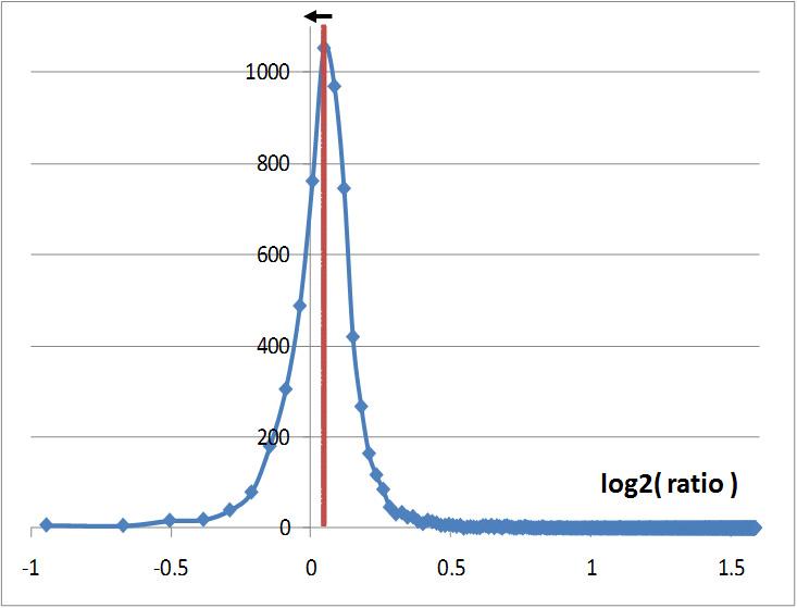
This last strategy has been published in 2006 (Dieterle, Ross et al. 2006) and gives the best results. It consists in calculating the intensity ratios between two maps to be compared then set the normalization factor as the inverse value of the median of these ratios (cf. figure below). The procedure is the following:
Distribution of the ratios transformed in log2 and calculated with the intensities of features observed in two LC-MS maps. The red line representing the median is slightly off-centered. The normalization factor is equal to the inverse of this median value. The normalization process will refocus the ratio distribution on 0 which is represented by the black arrow
Proline makes this normalization process for each match with the reference map and has a normalization factor for each map, independently of the choice of the algorithm. The normalization factor for the reference map is equal to 1.
This procedure is used to compute peptide and protein abundances. Several filters can also be set to increase the quality of quantitative results.
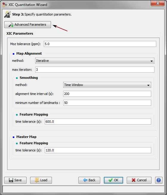
Here is the description of the parameters that can be modified by the user.
To calculate peptide abundance, associated peptides ions abundances can be summed or the best ion is used (the peptide ion with higher abundance).
Peptide abundances can be summarized into protein abundances using several mathematical methods:
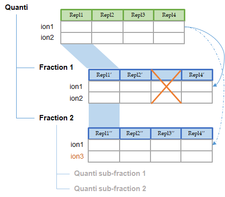
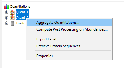
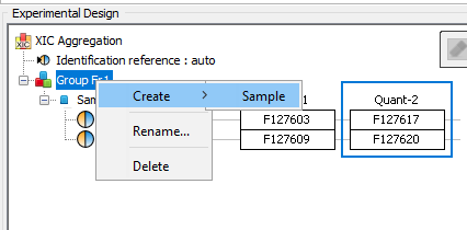
Two or more quantitations can be combined such that an ion quantified in multiple aggregated quantitations is represented only once in the aggregation result. The abundance of this ion is a combination of its abundance measured in the different aggregated quantitations. This could be useful to combine for example quantitation of fractions into a single quantitation result.
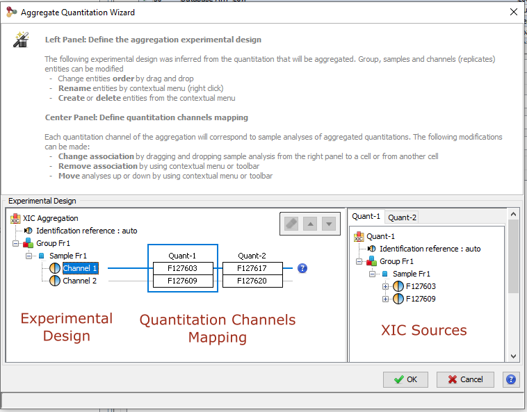
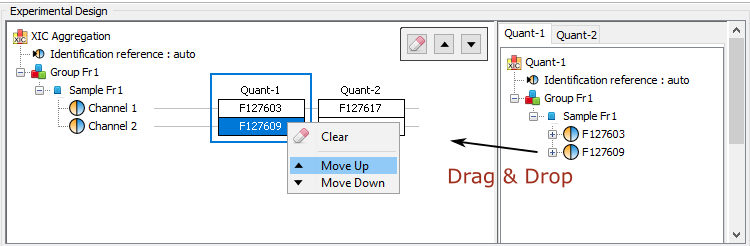
The experimental design of the aggregation is based on the experimental design of the aggregated quantitation: the number of group/condition and the number of replicates per condition remains the same. However, the user can modify the correspondence between the groups and replicates if needed. In the following example the abundance of ion1 in the aggregated quantitation (in green) is based on the quantitation of this same ion in "Fraction 1" and "Fraction 2". Since ion2 is quantified only in "Fraction 1", its abundance values in the aggregated quantitation are the same as the abundances measured in "Fraction 1".
In this simple example, the correspondence between experimental designs is such that the abundance of ion1 in the replicate Repl1 is based on the measured abundance of ion1 in Repl1’ in “Fraction 1” and Repl1’’ in “Fraction 2”. This could be modified by the user to take into account differences in the replicates order in aggregated quantitations or to account for the absence of a replicate (see for example replicate 3 in “Fraction 1”).
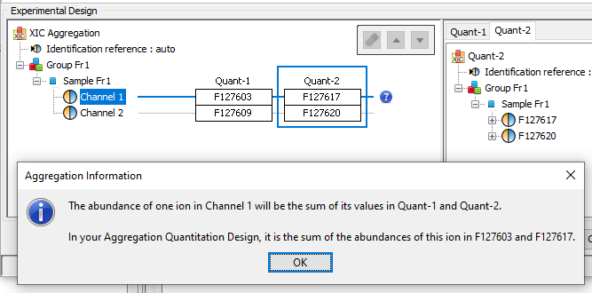
In the current version, the abundance at the aggregation level is the sum of the abundances in aggregated quantitations.
When exporting a whole Identification Summary in an excel file, the following sheets may be generated:
Raw2mzdb
The conversion is done using raw2mzDB.
Open a command line window in the directory containing raw2mzdb.exe
Enter:
raw2mzdb.exe -i <rawfilename> -o <outputfilename>
By default, the raw file will be converted in the “fitted” mode for the MS1 (MS2 is often in centroid mode and can not be converted in fitted mode). If the MS2 (or superior) are acquired in high resolution (i.e in profile mode), you could specify that you want to convert several MSs in the required mode: raw2mzdb.exe -i <rawfilename> -o <outputfilename> -f 1-2 will try to convert MS1 to MS2 in fitted mode.
There are two other available conversion modes:
Proline Studio
Note: Read the Concepts & Principles documentation to understand main concepts and algorithms used in Proline.
Calc. Mass: Calculated Mass
Delta MoZ: Delta Mass to Charge Ratio
Exp. MoZ: Experimental Mass to Charge Ratio
Ion Parent Int.: Ion Parent Intensity
Missed Cl.: Missed Cleavage
Modification D. Mass: Modification Delta Mass
Modification Loc.: Modification Location
Next AA: Next Amino-Acid
Prev. AA: Previous Amino-Acid
Protein Loc.: Protein Location of the Modification
Protein S. Matches: Protein Set Matches
PSM: Peptide Spectrum Match
PTM: Post Translational Modification
PTM D. Mass: PTM Delta Mass
RT: Retention Time
SC: Spectral Counting
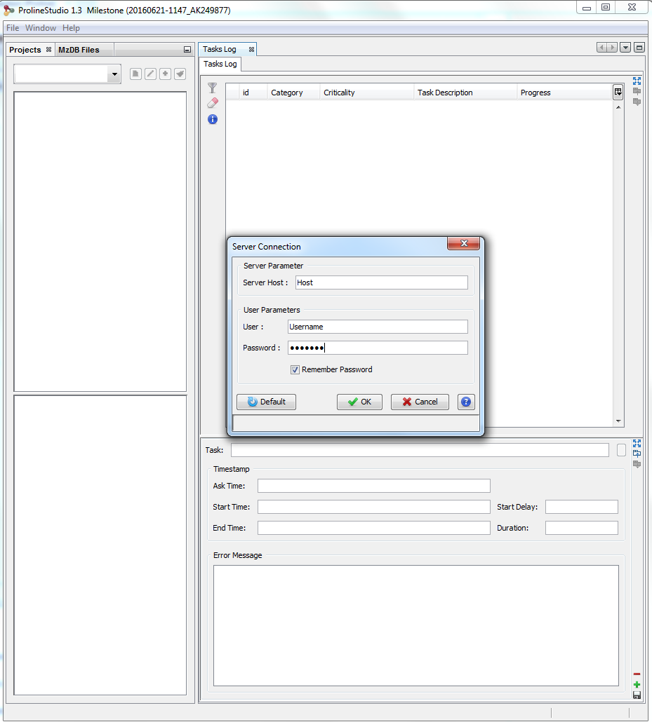
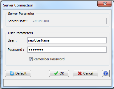
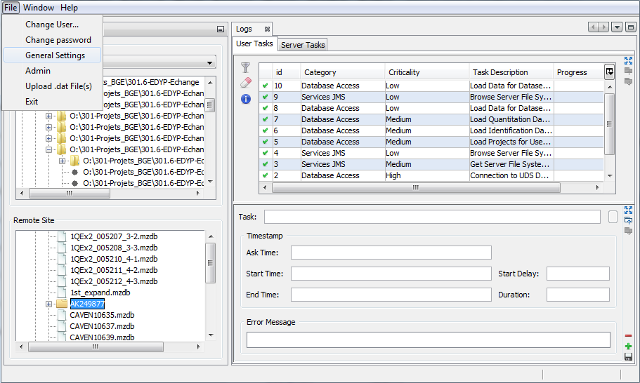
When you start Proline Studio for the first time, the Server Connection Dialog is automatically displayed.
You must fill the following fields:
- Server Host: this information must be asked to your IT Administrator. It corresponds to the Proline server name
- User: your username (an account must have been previously created by the IT Administrator).
- Password: password corresponding to your account (username).
If the field “Remember Password” is checked, the password is saved for future use. Server connection dialog continues to open with Proline Studio, the user though does not need to fill in his password, unless the last one is changed after his last login.
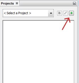
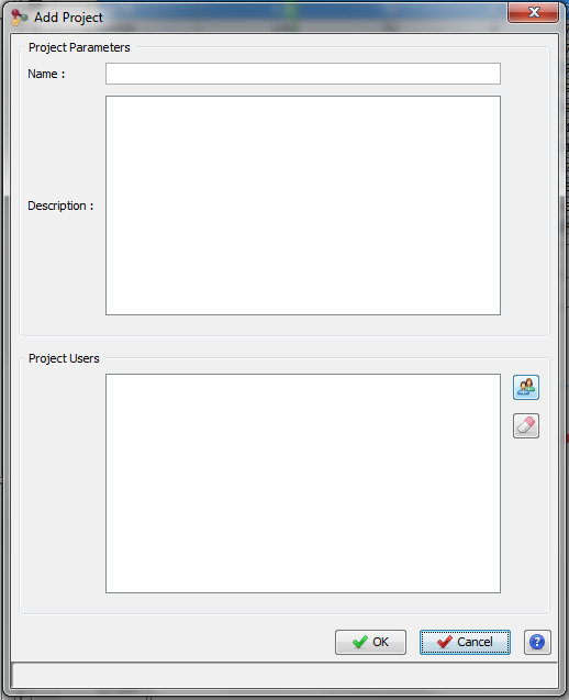
To create a Project, click on “+“ button at the right of the Project Combobox. The Add Project Dialog opens.
Fill the following fields:
- Name: name of your project
- Description: description of your project
You can specify other people to share this new project with them. Then click on OK Button
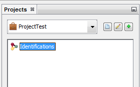
Creation of a Project can take a few seconds. During its creation, the Project is displayed grayed with a small hourglass over it.
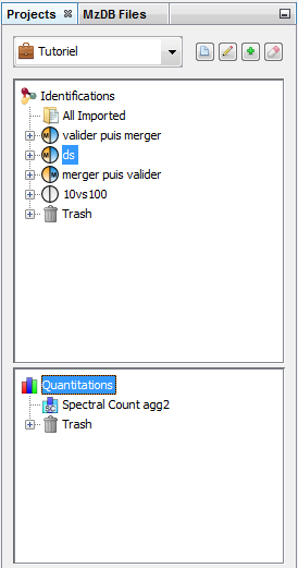
In the Identification tree, you can create a Dataset to group your data
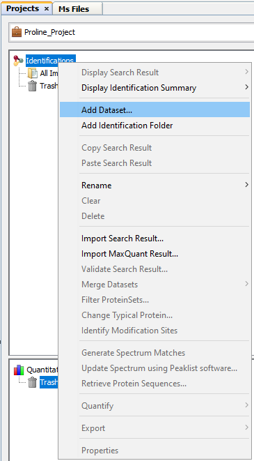
To create a Dataset:
- right click on Identifications or on a Dataset to display the popup.
- click on the menu “Add Dataset…”
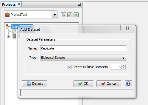
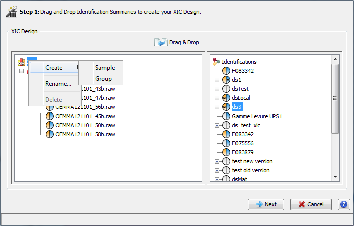
On the dialog opened:
- fill the name of the Dataset
- choose the type of the Dataset
- optional: click on “Create Multiple Datasets” and select the number of datasets you want to create
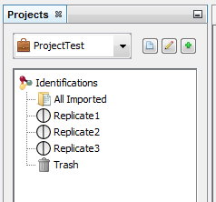
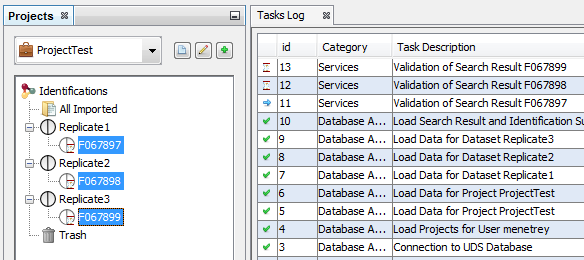
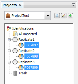
Let's see the result of the creation of 3 datasets named “Replicate”:
In both Identification and Quantitation tree, you can create Folders to organize your data
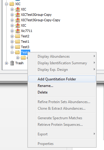
To create a Folder :
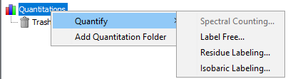
- right click on Identifications, Quantitations or on a Folder to display the popup.
- click on the menu “Add Identification Folder…” or “Add Quantitation Folder…”
See Concept & Principle section
There are two possibilities to import Search Results:
- import multiple Search Results in “All Imported” and put them later in different datasets.
- import directly a Search Result in a dataset.
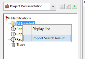
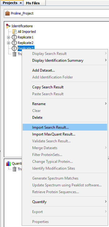
To import in “All Imported”:
- right click on “All Imported” to show the popup
- click on the menu “Import Search Result…”
It is possible to import Search Results directly in a Dataset. Even in this case, Search Results are available in “All Imported”.
To import a Search Result in a Dataset, right click on a dataset and then click on “Import Search Result…” menu. Same dialog and parameters as in “Import in “All Imported”” above will be displayed. |
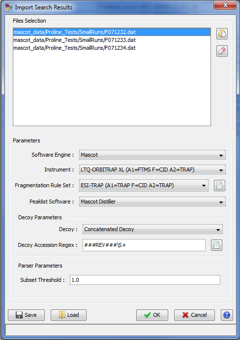
In the Import Search Results Dialog:
- select the file(s) you want to import thanks to the file button (the Parser will be automatically selected according to the type of file selected)
- select the different parameters (see description below)
- click on OK button
Note 1: You can only browse the files accessible from the server according to the configuration done by your IT Administrator. Ask him if your files are not reachable. (Look for Setting up Mount-points paragraph in Installation & Setup page).
Note 2: Proline is able to import OMSSA files compressed with BZip2.
Parameters description:
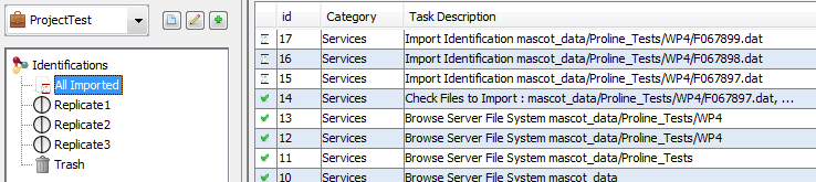
Importing a Search Result can take some time. While the import is not finished, the “All Imported” or “selected dataset” is shown grayed with an hourglass and you can follow the imports in the Tasks Log Window (Menu Window > Tasks Log to show it).
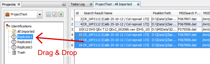
To show all the Search Results imported, double click on “All Imported”, or right click to popup the contextual menu and select “Display List”
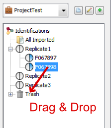
If needed, from the All Imported window, you can drag and drop one or multiple Search Result to an existing dataset.
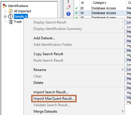
To import a MaxQuant Search Result, right click on a dataset and then select “Import MaxQuant”
Note 1: MaxQuant import will generate a dataset hierarchy with the result from the different acquisition.
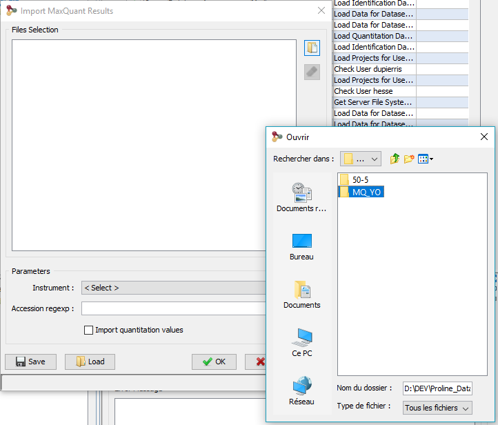
The following dialog will be displayed
- select the directory containing the files generated by MaxQuant. This folder should look like:
<root_folder>\mqpar.xml
<root_folder>\combined\txt\summary.txt
<root_folder>\combined\txt\proteinGroups.txt
<root_folder>\combined\txt\parameters.txt
<root_folder>\combined\txt\msmsScans.txt
<root_folder>\combined\txt\msms.txt
- select the Instrument: mass-spectrometer used for sample analysis different parameters
- specify, if needed, the regular expression to extract protein accessions from MaxQuant protein ids.
- you can choose to import also quantitative data
- click on OK button
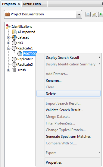
You can delete Search Results, Identification Summaries and Datasets in the data tree. You can also delete XIC or Spectral Counts in the quantitation tree.
Delete the Datasets (identification or quantitation…) from the tree view (Search Result always accessible from “All Imported” view…).
There are two ways to delete data: use the contextual popup or drag and drop data to the Trash.
Select the data you want to delete, right-click to open the contextual menu and click on delete menu.
The selected data is put in the Trash. So it is possible to restore it while the Trash has not been emptied.
Select the data you want to delete and drag it to the Trash. It is possible to restore data while the Trash has not been emptied
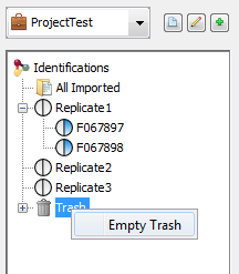
To empty the Trash, you have to Right click on it and select the “Empty Trash” menu.
A confirmation dialog is displayed and if accepted Dataset will be removed from the Trash.
Search Results are not completely removed, you can retrieve them from the “All Imported” window.
It is not possible to delete a Project by yourself. If you need to do it, ask your IT Administrator.
Once user is connected (see Server Connection), it is possible to:
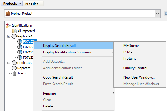
All information, validated or not, can be accessible from this menu. Indeed, Search Result contains all data imported from a result file without any validation consideration.
To display data of a Search Result:
- right click on a Search Result
- click on the menu “Display Search Result >” and on the sub-menu “MSQueries” or “PSM” or “Proteins”
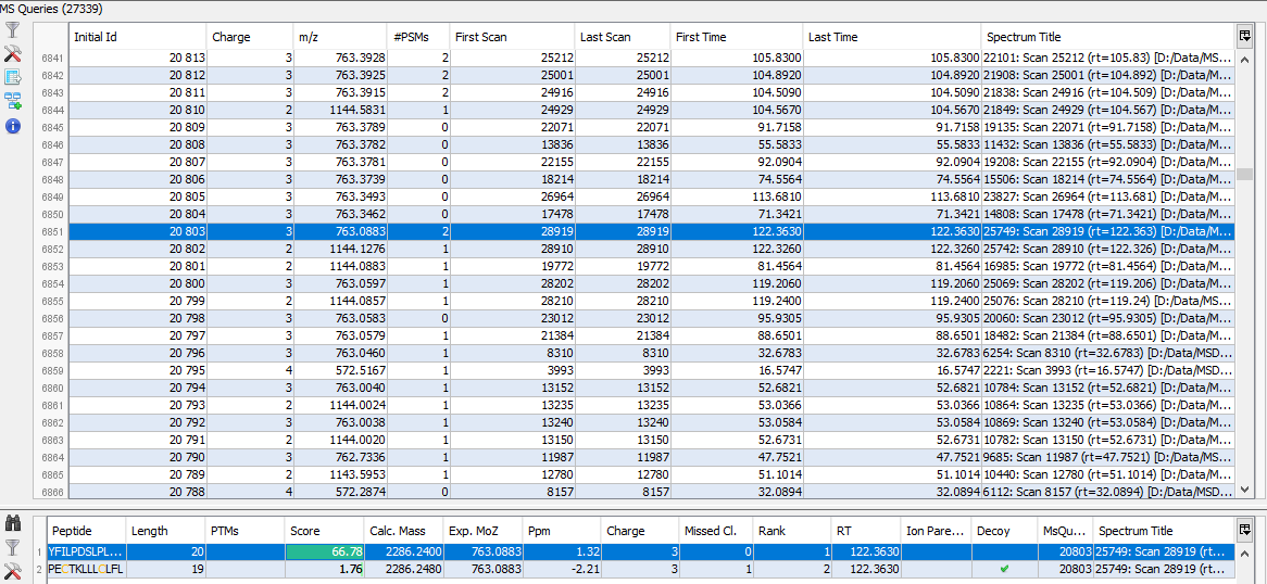
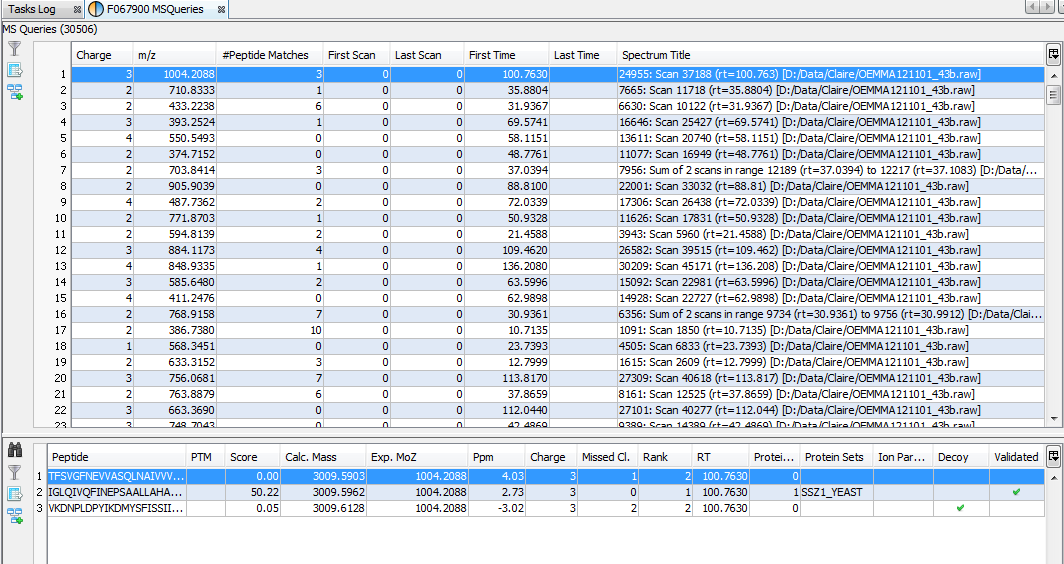
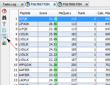
If you click on MSQueries sub-menu, you obtain this window:
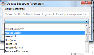
Upper View: list of MSQueries. Some columns may not be (correctly) filled if the Peaklist software were not correctly specified during import. It is possible to change this information using ‘Update Spectrum ..’
Bottom Window: list of all Peptides linked to the current selected MSQuery.
Note: Abbreviations used are listed here
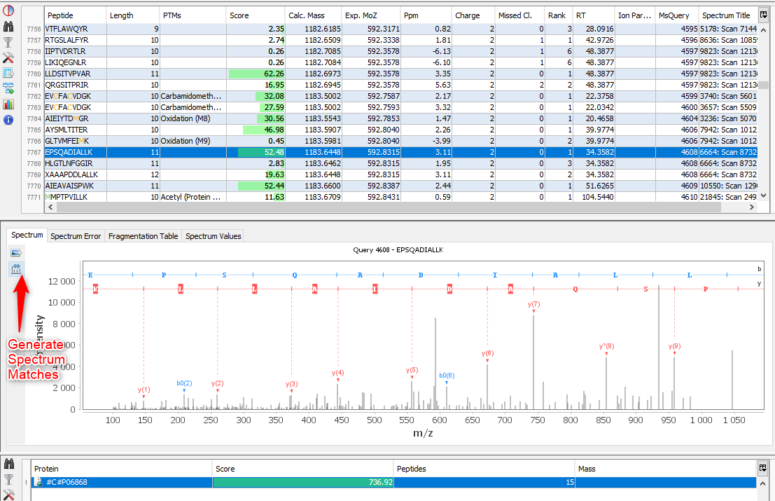
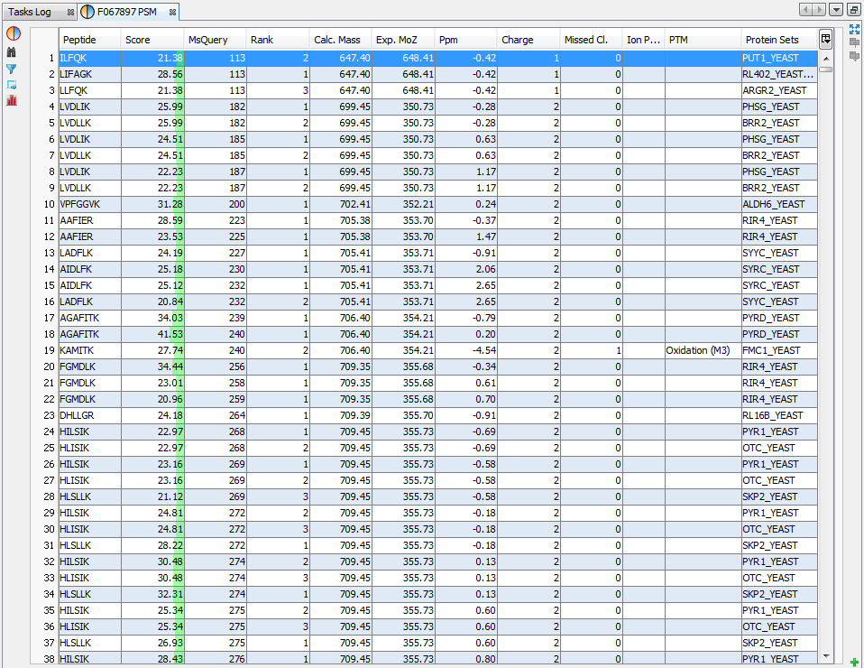
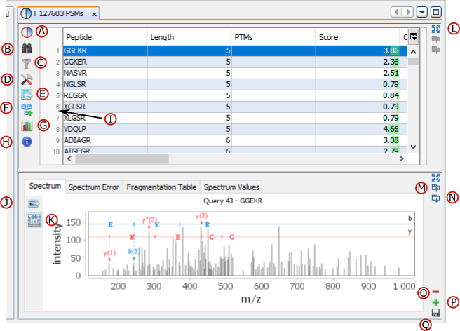
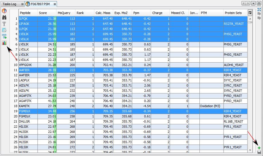
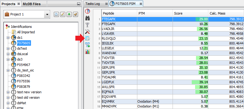
If you click on PSMs sub-menu, you obtain this window:
Upper View: list of all Peptide Spectrum Matches
Middle View: Spectrum, Spectrum Error , Spectrum Values and Fragmentation Table of the selected PSM. If no annotation is displayed, you can generate Spectrum Matches by clicking on the according button
Bottom Window: list of all Proteins identified by the currently selected Peptide.
Note: Abbreviations used are listed here
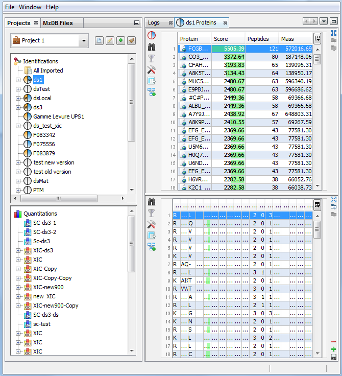
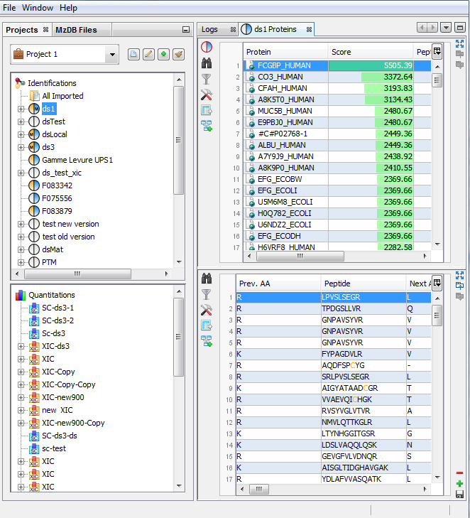
If you click on Proteins sub-menu, you obtain this window:
Upper View: list of all Proteins
Bottom View: list of all Peptides identifying the selected Protein.
Note: Abbreviations used are listed here
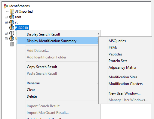
From this menu, all displayed information is Identification Summary data, which has been validated according to user specified rules. To view the raw information as defined at import, use the Search Result sub menu.
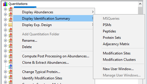
To display data of an Identification Summary:
- right click on an Identification Summary
- click on the menu “Display Identification Summary >” and on the sub-menu “MSQueries”, “PSM”, “Peptides”, “Protein Sets”, “PTM Protein Sites” or “Adjacency Matrix”
If you click on MSQueries sub-menu, you obtain this window:
Upper View: list of MSQueries.
Bottom Window: list of all Peptides linked to the current selected MSQuery.
Note: Abbreviations used are listed here
This view contains all MSQueries even if it doesn’t bring an identification.
If you click on PSM sub-menu, you obtain this window:
Note: Abbreviations used are listed here
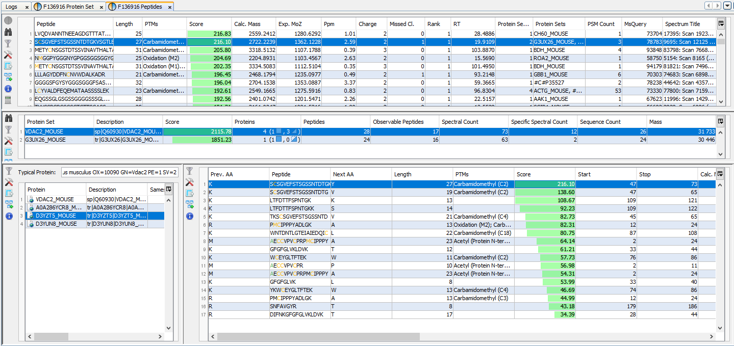
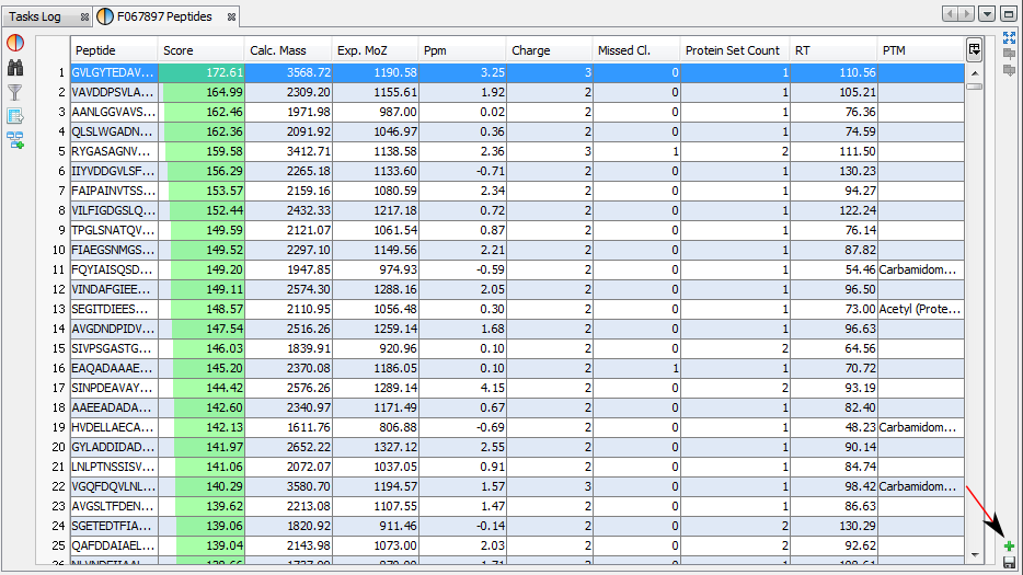
If you click on Peptides sub-menu, you obtain this window:
Upper View: list of all Peptides with best PSM information (charge, score ...)
Middle View: list of all Protein Sets identified by the selected peptide.
Bottom Left View: list of all Proteins of the selected Protein Set
Bottom Right View: list of all Peptides of the selected Protein
Note: Abbreviations used are listed here
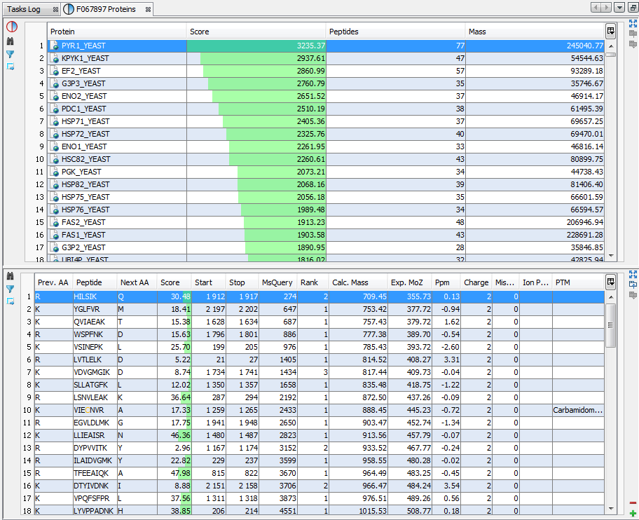
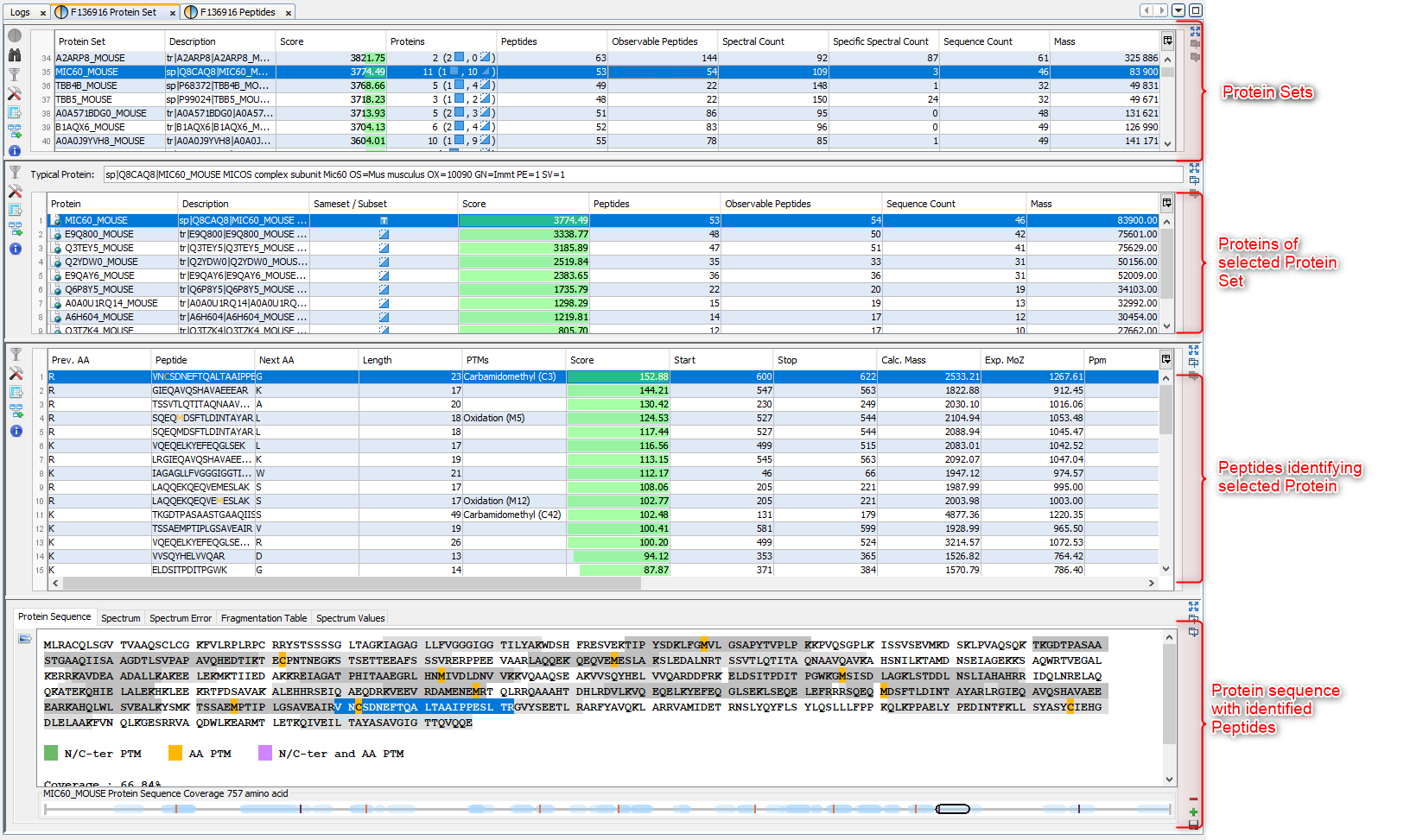
If you click on Protein Sets sub-menu, you obtain this window:
View 1 (upper): list of all Protein Sets of the identification Summary
Note: In the column Proteins, 8 (2, 6) means that there are 8 proteins in the protein set : 2 in the sameset, 6 in the subset.
View 2: list of all Proteins of the selected Protein Set, sameset or subset.
View 3: list of all Peptides of the selected Protein. If a subset is selected only peptides matching that protein will be listed.
View 4a: Protein Sequence of the previously selected Protein and Spectrum of the selected Peptide. Other tabs display Spectrum, Spectrum Error and Fragmentation Table.
View 4b: Graphic representation of the Protein with matching peptide and associated modifications.
Note: Abbreviations used are listed here
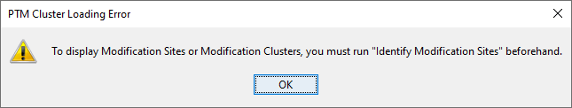
If you click on Modification Sites or Modification Clusters sub-menu, you could obtain the following warning dialog.
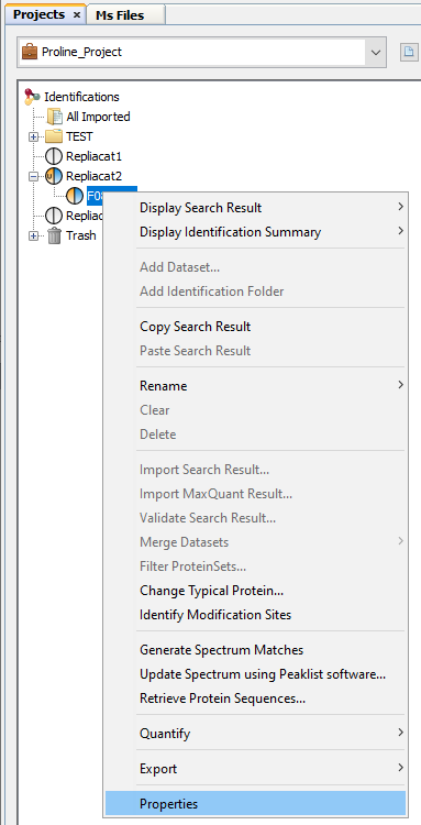
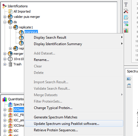
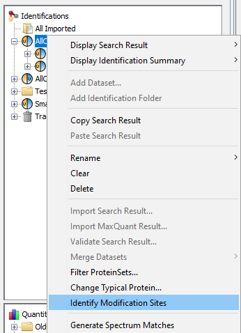
This is due to the fact that you must run beforehand the “Identify Modification Sites” process. To do that, mouse right click on your Identification Summary and select “Identify Modification Sites” menu.
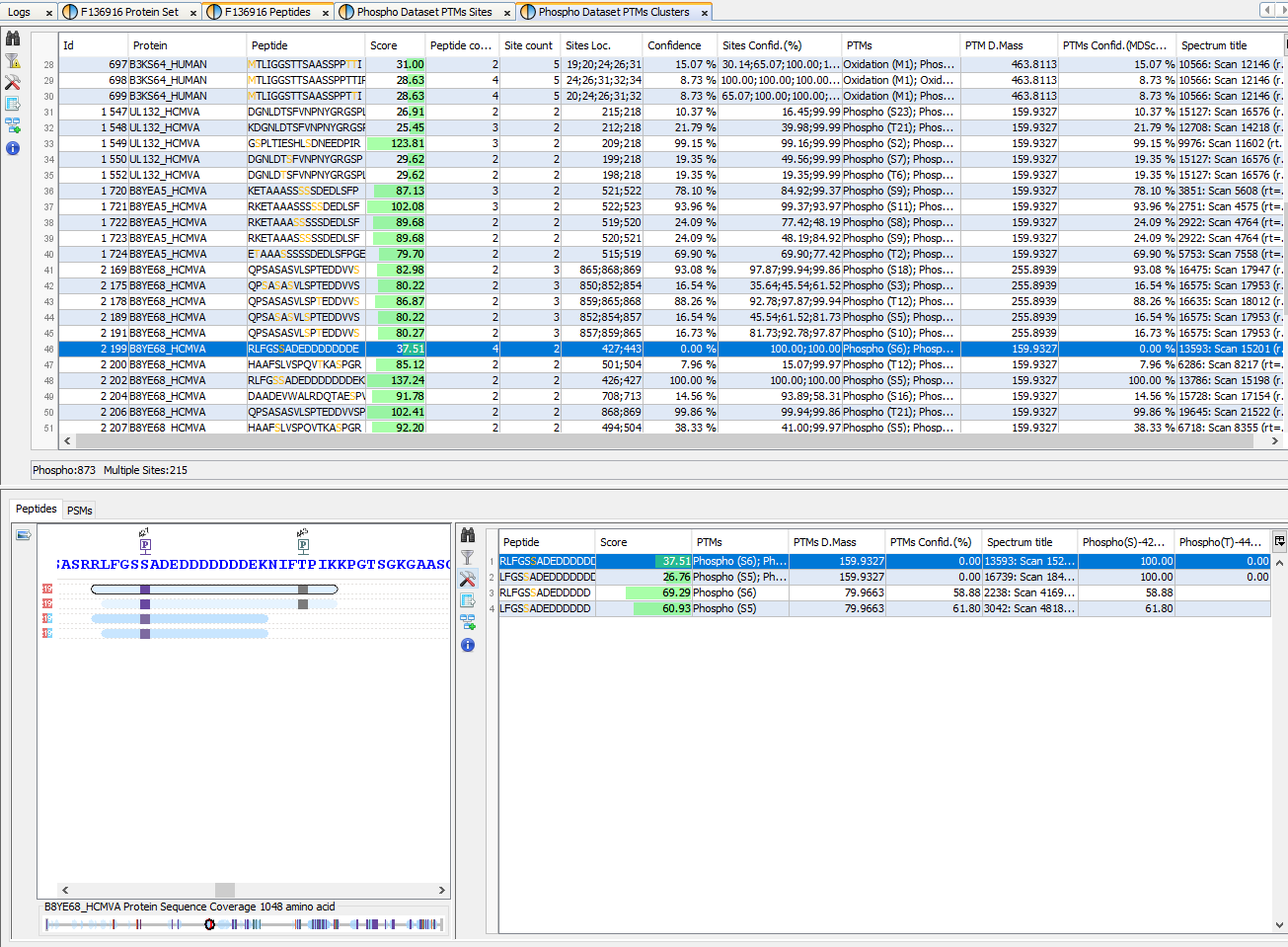
Both display, Sites and Clusters, are structured in the same way. In Sites windows, the upper view will list all individual Sites (a specific modification at a specific location for a given Protein) while in Clusters windows, Sites will be clustered using rules specified by user (see Identify Modification Sites)
Upper View: This view lists all Modification Sites or Clusters. In this example, a Cluster view is shown. For each of them, many information is given : the number of Peptides belonging to the Cluster, how many sites have been clustered, The Confidence for the site combination, ...
Bottom Left view: Graphic illustration of the cluster/site peptides mapped to the protein sequence. All modification locations are represented above the protein sequence. An overview graphic is also given below.
Bottom Right view: Cluster/Site peptides list. The PSMs list is accessible in a hidden tab.
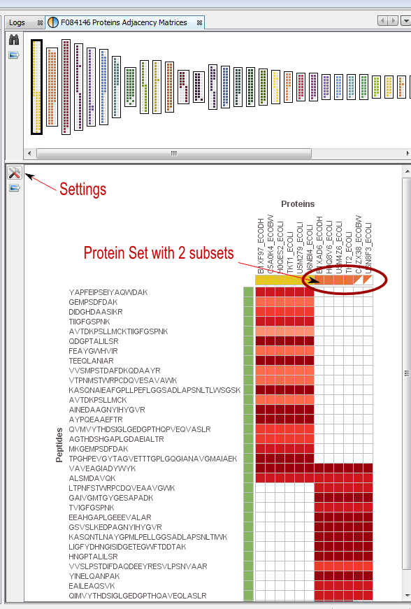
If you click on Adjacency Matrix sub-menu, you obtain this window:
View 1: All the matrices. Each matrix corresponds to a cluster composed of linked Proteins/Peptides.
Note: use the Search tool to display an Adjacency Matrix for a particular Protein or Peptide
View 2: The currently selected matrix.
In the example, you can see two different protein sets which share only two peptides.
Thanks to the settings you can hide proteins with exactly the same peptides.
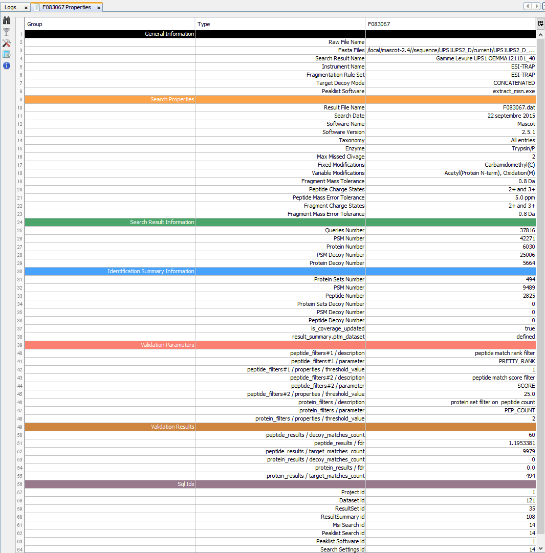
To display properties of a Search Result or Identification Summary:
Note: it is possible to select multiple Search Results/Identification Summaries to compare the values.
Property window opened:
General Information: Various information on the analysis (instrument name, peaklist software…)
Search Properties: Information extracted from the Result File (date, software version, search settings...)
Search Result Information: Amount of Queries, PSM and Proteins in the Search Result.
Identification Summary Information: Information obtained after validation process
Validation xxx: Information on validation process : parameters used to validate and result
Sql Ids: Database ids related to this item
Note: Identification Summary Number may differ from Validation Results. Indeed, on one hand, peptide matches count in Validation Results takes into account all PSMs that have been validated . On the other hand, the PSM Number in “Identification Summary Information” section considers only PSMs that identify a valid Protein Sets.
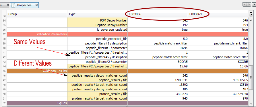
Property window opened with multiple Identification summaries selected:
The color of the type column indicates if the values are the same (white) or different (yellow)
.
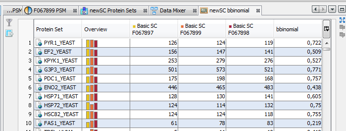
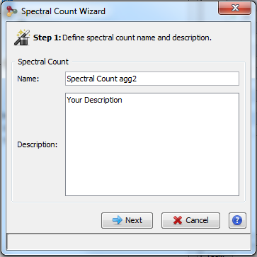
You can display a generated Spectral Count by using the right mouse popup.
To have more details about the results, see spectral_count_result
The overview is based by default on the weighted spectral count values. (Note: if you sort on the overview column, the sort is based on max (value-mean (values))/mean (values). So, you will obtain the most homogenous and confident rows first)
For each compared dataset, are displayed:
- status ( typical, sameset, / )
- peptide numbers
- the basic spectral count
- the specific spectral count
- the weighted spectral count
- the selection level
User can change the information displayed by the overview using the table settings icon ( ) .
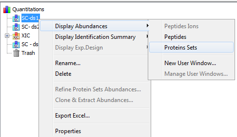
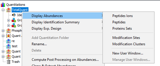
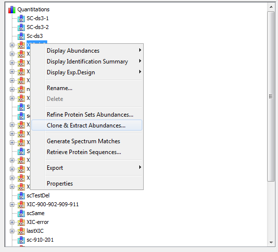
To display a XIC, right click on the selected XIC node in the Quantitation tree, and select “Display Abundances”, and then the level you want to display:
Note: You can also display the identification summary used as reference for the quantitation from the popup menu in the quantitation tree:
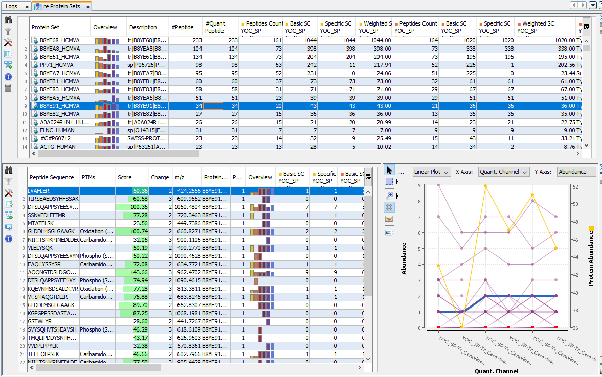
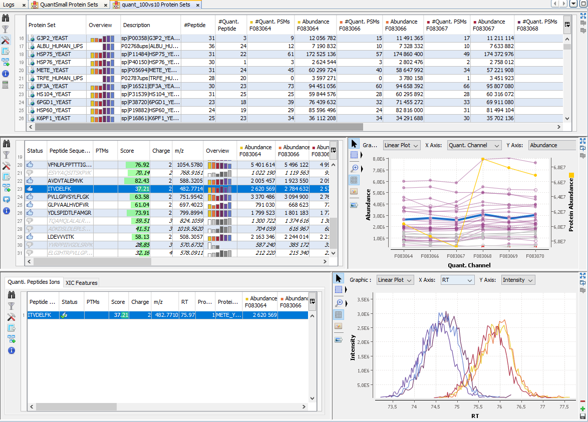
By clicking on “Display Abundances” / “Protein Sets”, you can see all quantified protein sets. For each quantified protein set, you can see below all peptides linked to the selected protein set and peptides Ions linked to the selected peptide. For each peptide Ion, you can see the different features and the graph of the peakels in each quantitation channel.
The overview is based by default on the abundances values.
Note: if you sort on the overview column, the sort is based on max (value-mean (values))/mean (values). So, you obtain the most homogenous and confident rows first.
For each quantitation channel, are displayed:
- the raw abundance
- the peptide match count
- the abundance
- the selection level
By clicking on the using the “table setting” icon , you can choose the information you want to display or change the overview.
The middle part of the window lists all peptides of the selected Protein set with the same kind of quantitative data. The status column indicates whether the peptide was used or not for protein set abundances. On the right part, a graph allows you to see the variations of the abundance (or raw abundance) of a peptide in the different quantitation channels.
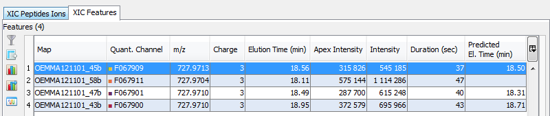
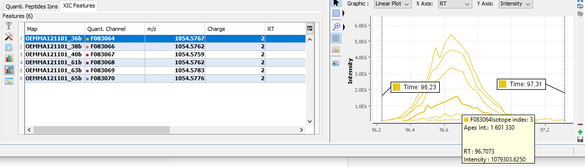
You can see the different features in the different quantitation channels and the graph of the peakels:
By clicking on you can display either:
- the peaks of isotope 0 in all quantitation channels
- all isotopes for the selected quantitation channel:
By clicking on you can see the chromatograms of the features and their first time scan and last time scan in mzScope. For more details see the mzScope section.
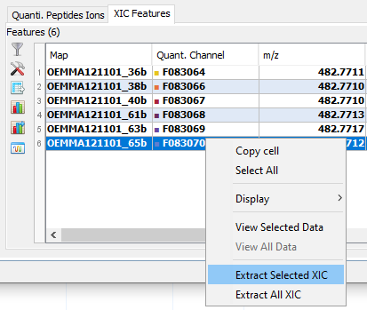
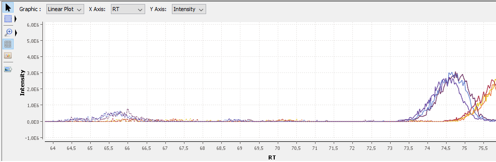
It is also possible to extract the corresponding chromatogram for one or all of the features.
The resulting chromatograms will be displayed in the same windows as peakel.
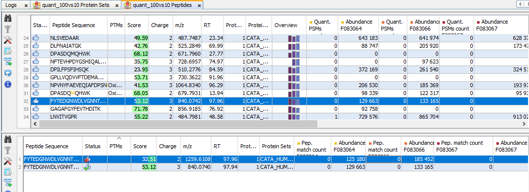
By clicking on “Display Abundances“ / “Peptides”, you can see:
- identified and quantified Peptides
- non identified but quantified peptides
- identified but not quantified peptides (linked to a quantified protein)
The lower view lists all peptide ions (specific charge) of selected peptide. The status column indicates if the ion is valid or not and if it was used for peptide quantitation.
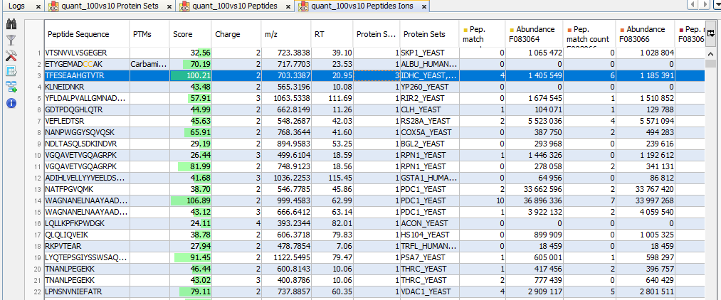
By clicking on “Display Abundances” / “Peptides Ions”, you can see:
- all identified and quantified Peptides Ions
- non identified but quantified peptides Ions
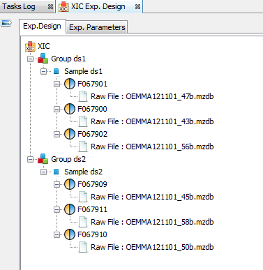
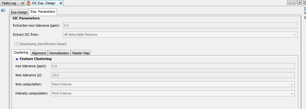
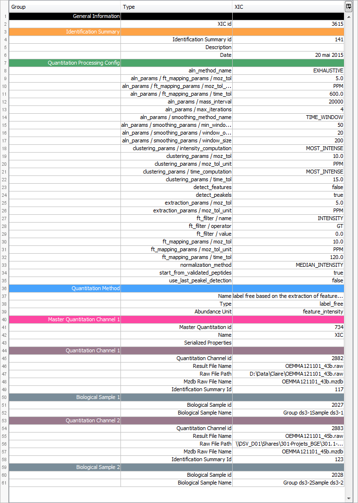
By clicking on “Exp. Design > Parameters”, you can see the experimental design and the parameters of the selected XIC.
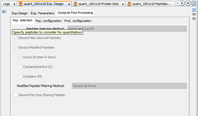
If you have launched the “compute post processing ...” on the XIC, you can also display the corresponding parameters.
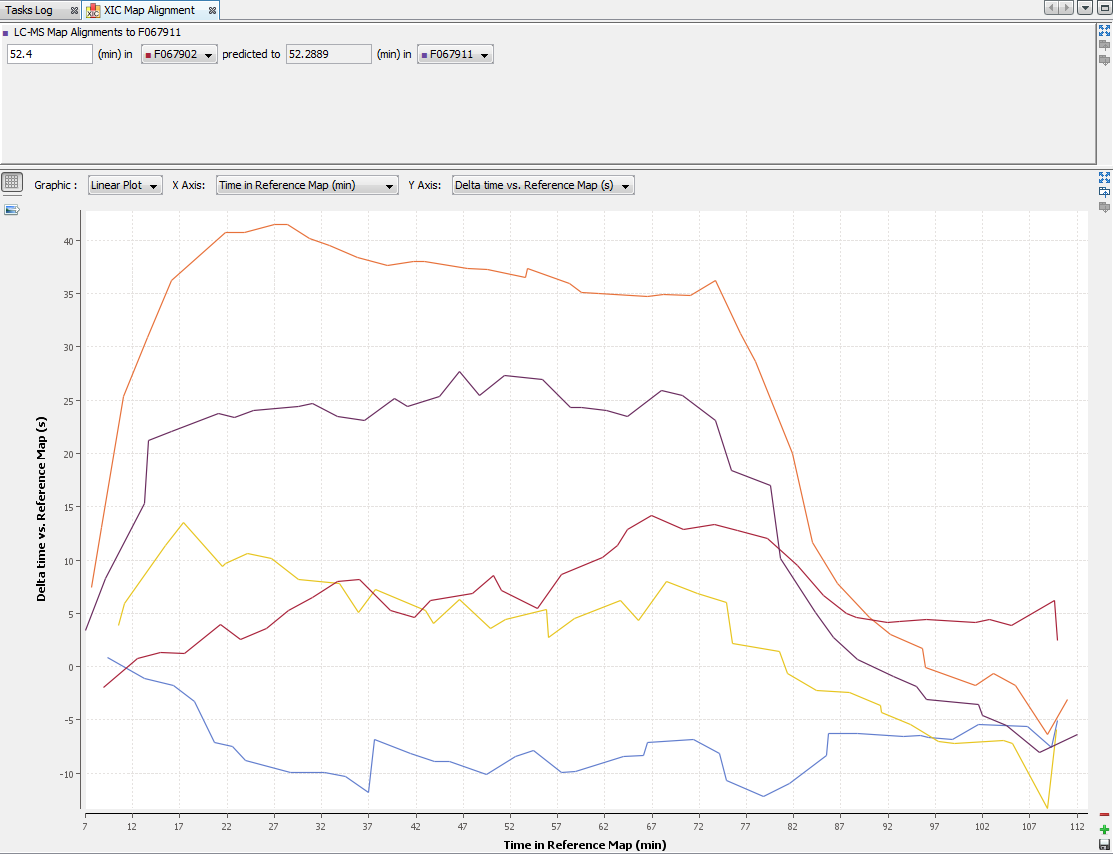
By clicking on “Exp. Design > Map Alignment”, you can see the map of the variation of the alignment of the maps compared to the map alignment of the selected XIC. You can also calculate the predicted time in a map from an elution time in another map.
A: Display Decoy Data.
B: Search in the Table. (Using * and ? wild cards)
C: Filter data displayed in the Table
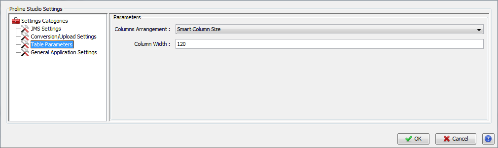
D: Display settings dialog (you can modify displayed columns and perform double sorting)
E: Export data displayed in the Table
F: Send to Data Analyzer to compare data from different views
G: Create a Graphic : histogram or scatter plot . Only on PSMs table
H: Display number of entities in the table (number of PSMs / Peptides / Proteins…)
I: Right click on the marker bar to display Line Numbers or add Annotations/Bookmarks
J: Export view as an image
K: Generate Spectrum Matches (specific to spectrum grahic)
L: Expands the frame to its maximum (other frames are hidden). Click again to undo.
M: Gather the frame with the previous one as a tab.
N: Split the last tab as a frame underneath
O: Remove the last Tab or Frame
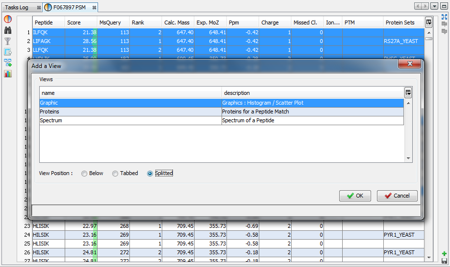
P: Open a dialog to let the user add a View (as a Frame, a Tab or a splitted Frame)
Q: Save the window as a user window, to display the same window with different data later
You can lay out your own user window with the desired views.
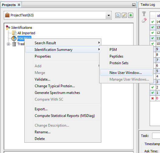
You can do it from an already displayed window, or by using the right click mouse popup on a dataset like in the following example (Use menu “Search Result>New User Window…” or “Identification Summary>New User Window…”)
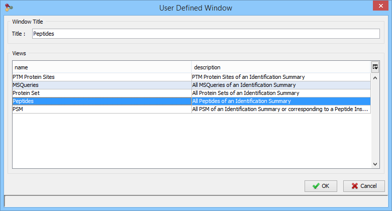
In the example, the user has clicked on “Identification Summary>New User Window…” and selects the Peptides View as the first view of his window.
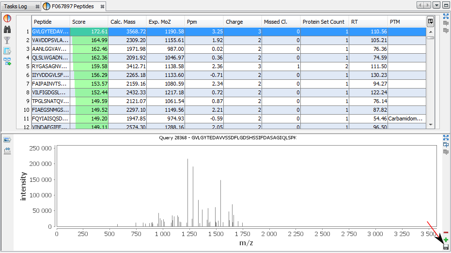
You can add other views by using the '+' button.
In this example, the user has added a Spectrum View and he saves his window by clicking on the “Disk” Button.
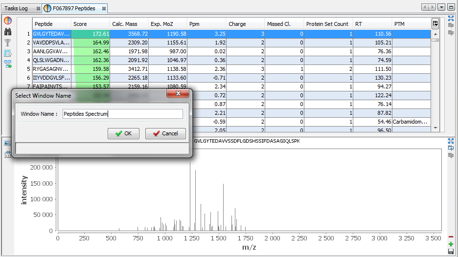
The user selects 'Peptides Spectrum' as his user window name
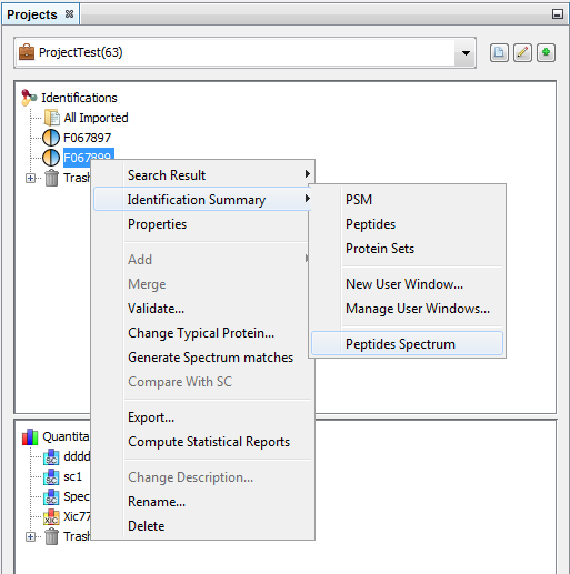
Now, the user can use his new 'Peptides Spectrum' on a different Identification Summary.
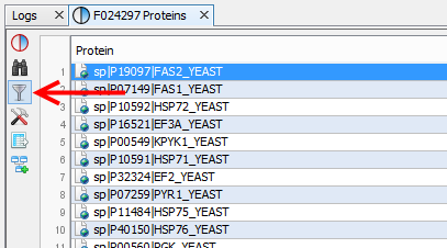
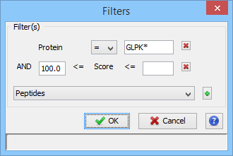
You can filter data displayed in the different tables thanks to the filter button at the top right corner of a table.
When you have clicked on the filter button, a dialog is opened. In this dialog you can select the columns of the table you want to filter thanks to the “+” button.
In the following example, we have added two filters:
- one on the Protein Name column (available wildcards are * to replace multiple characters and ? to replace one character)
- one on the Score Column (Score must be at least 100 and there is no maximum specified).
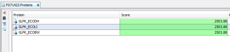
The result is all the proteins starting with GLPK (correspond to GLPK*) and with a score greater or equal than 100.
Note: for String filters, you can use the following wildcards: * matches zero or more characters, ? matches one character.
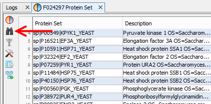
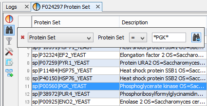
In some tables, a Search Functionality is available thanks to the search button at the top right corner.
When you have clicked on the search button, a floating panel is opened. In this panel you can select the column searched and fill in the searched expression, or the value range.
For searched expressions, two wild cards are available:
In the following example, the user searches for a protein set whose name contains “PGK”.
You can do an incremental search by clicking again on the search button of the floating panel, or by pressing the Enter key.
There are two ways to obtain a graphic from data:
If you have clicked on the '+' button, the Add View Dialog is opened and you must select the Graphic View
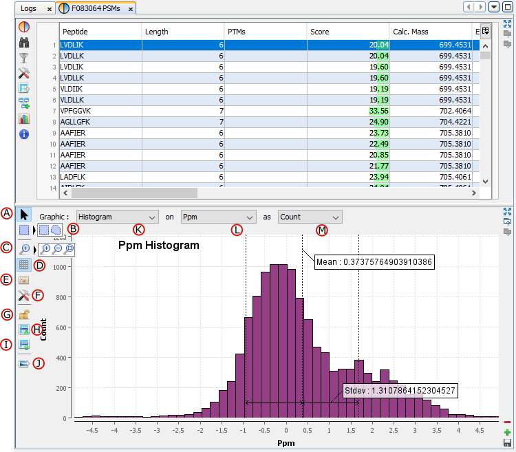
A: When this button is selected, you have the “Pointer Mode” activated.
In this mode :
- If you move with the left mouse button pressed on the middle of the graphic, you can scroll along the X and Y Axis.
- If you move with the right mouse button pressed from the top/left corner to the bottom/right corner, a zooming rectangle is displayed. When you release the mouse button, a zoom in according to the zooming rectangle is performed.
- If you move with the right mouse button pressed from the bottom/right corner to the left/top corner, a view all is done.
B: When this button is selected, you have the “Selection Mode” activated.
By clicking on the black right arrow, you can switch between the square selection mode and the lasso selection mode.
In this mode:
C: Zoom out / Zoom in / View all. Click on the black right arrow to select the zooming mode.
D: Display/Remove Grid toggle button
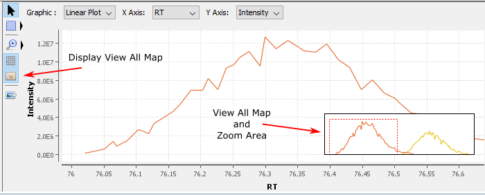
E: Display/Hide View All Map. The goal of this map is to display the whole graphic in a small zone even when you have zoomed
F: Open a settings dialog for the graphic. You can modify for example colors or bins of an histogram.
G: Lock/Unlock incoming data. If it is unlocked, the graphic is updated when the user applies a new filter to the previous view (for instance Peptide Score >= 50) If it is locked, changing filtering on the previous view does not modify the graphic.
H: Select Data in the graphic according to data selected in the table in the previous view.
I: Select data in the table of the previous view according to data selected in the graphic.
J: Export graphic to image
K: Select the graphic type: Scatter Plot / Histogram
L/M: Select data used for X / Y axis.
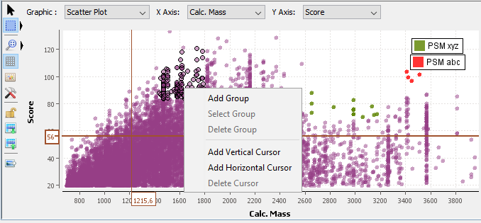
By right mouse click on the graphic area, you get a popup with several menus:
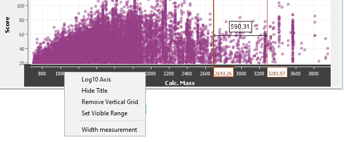
By right mouse click on an axis, you get a popup with several menus:
There are several ways to perform zoom actions.
Zoom in:
Zoom out:
View All:
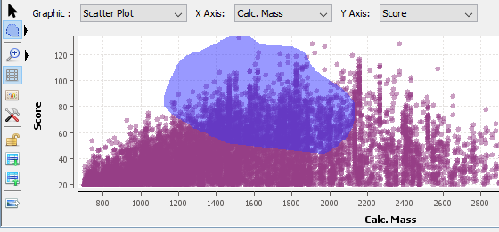
To be able to select data, you must be in “Selection Mode”
Select: You can select with a rectangle area or with a lasso according to the selected button. Press the left mouse button and drag the mouse to surround the data you want to select. When you release the button, the selection is done. Or left click on the data you want to select. It is possible to use the Ctrl key to add to the previous selection.
Unselect: Left click on an empty area to clear the selection.
Click on View All Map button to display the map. This map always displays the whole graphic and the zoomed area. You can directly zoom on the view all map. You can resize it and move it.
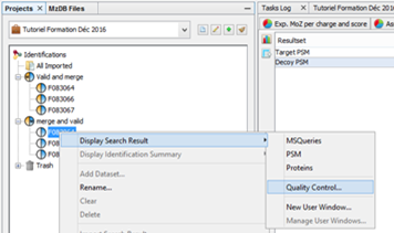
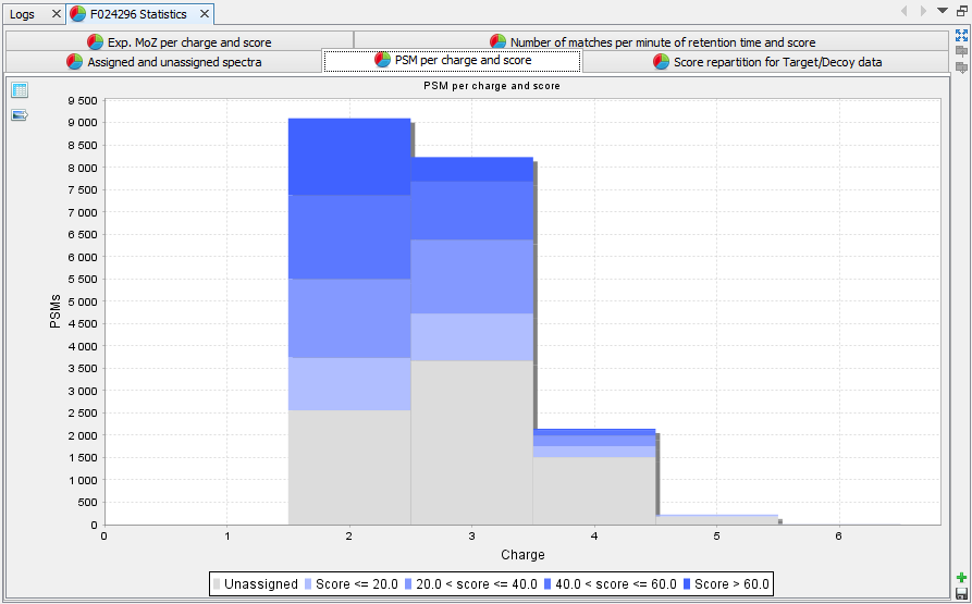
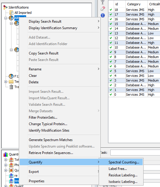
You can run a Quality Control on any leaf Search Result, that is to say an imported Result File not a merged search result. It consists in a transversal view of the imported data: rather than visualising the results per PSM or Proteins, results are sorted according to the score, charge state...
Choose the menu option:
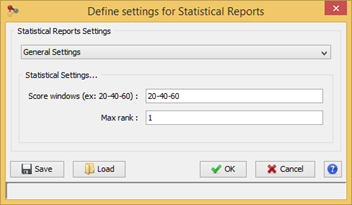
Configure some settings before launching the process
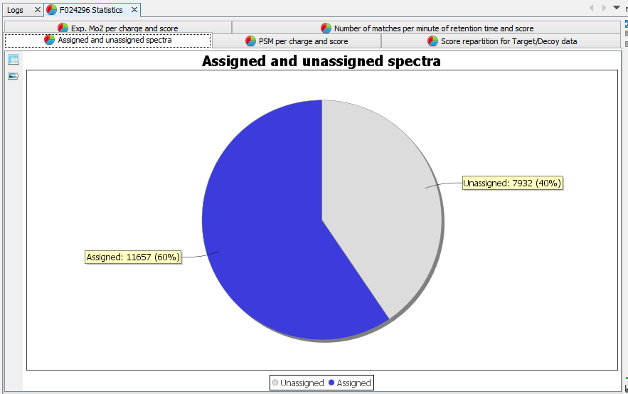
The report will appear in a matter of seconds (depending on the amount of data to be processed). You will get the following tabs:
Assigned and unassigned spectra: Pie chart presenting the ratio of assigned spectra | |
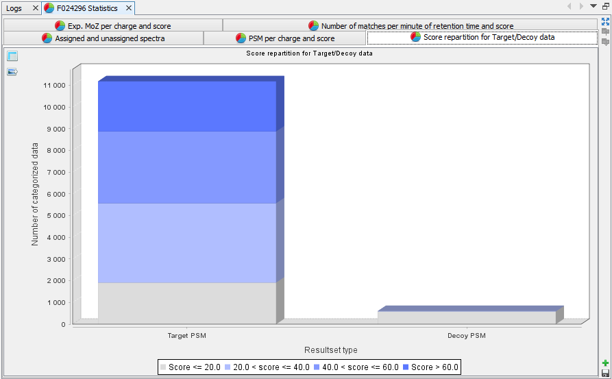
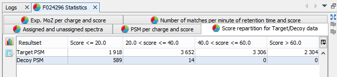
Score repartition for Target/Decoy data: Histogram presenting the amount of PSM per group of score, separating target and decoy data | |
PSM per charge and score: Histogram presenting the amount of PSM per group of score and charge state | |
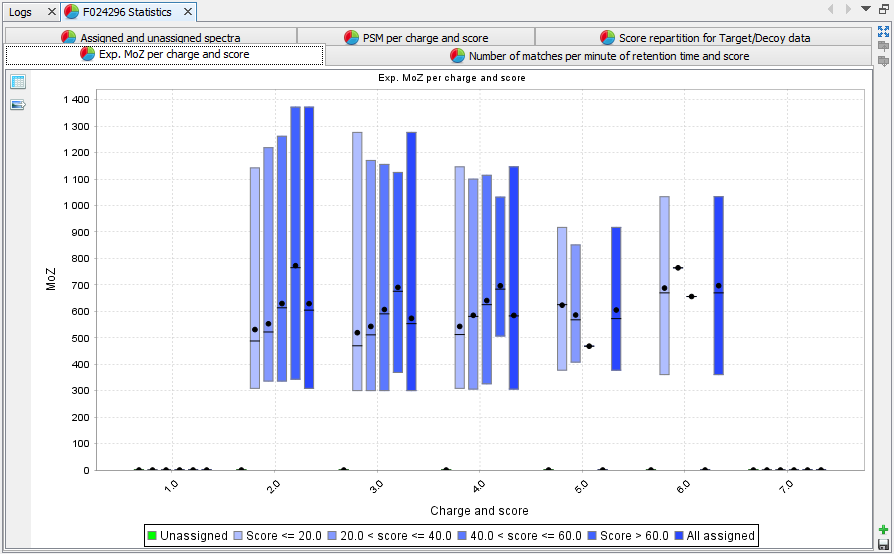
Experimental M/z per charge and score: Box plot presenting M/z information for each category of score and charge state | |
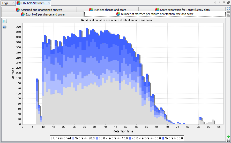
Number of matches per minute of RT and score: histogram presenting the amount of PSM per score and retention time. This view is only calculated when retention time is available. | |
Each graph is also available in a table view |
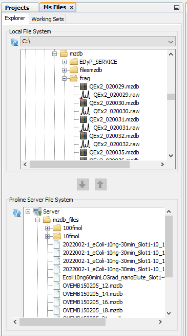
In order to facilitate different actions on Ms Files, Proline Studio contains an homonym tab providing the end user with a view over his local and server remote file system, called Local File System and Proline Server File System respectively.
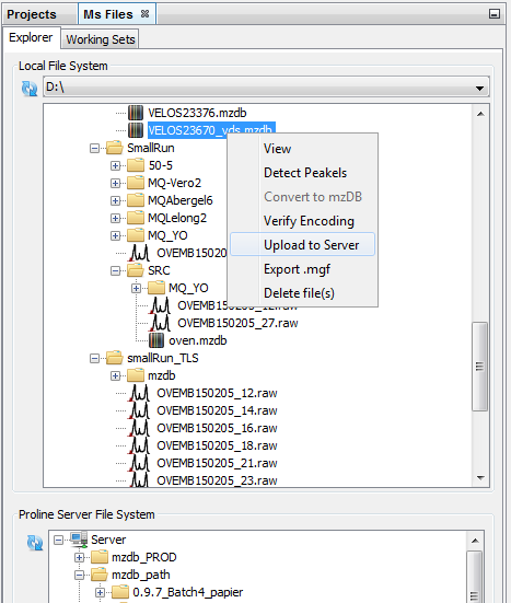
Furthermore, on local file system a series of actions can take place, through an appropriate popup menu, on the encountered .mzdb and .raw files, including among others the:
Apart from the popup menu supported functionality, since Proline Studio 1.5, uploads can be triggered via drag and drop mechanism.
As mentioned earlier, after selecting a number of files, the user can either drag and drop them inside the remote site, or use the popup menu as shown in the following screenshot. It is important to precise that both approaches are not compatible with a selected group consisting of different file types.
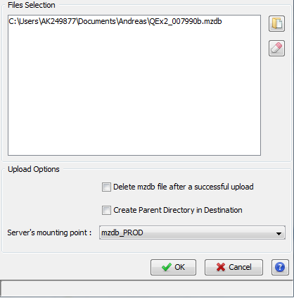
As we can see, clicking on upload opens a dedicated dialog packing a series of uploading options:
Furthermore, the dialog permits us to add or remove .mzdb files to upload. The uploading tasks status could be viewed in the Logs tab.
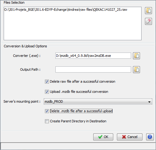
In the same way, when the user desires to convert and upload a raw file, he or she can either drag and drop it on the Remote Site view, or use the respective dialog through the popup menu.
For the upload step, the same options as described above are shown.
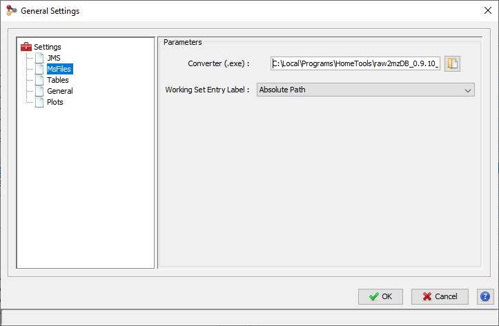
For the conversion, the path to the converter exe file should be specified. This value will be saved upon different executions. A default path may be specified in the general settings dialog. The same way .mzdb file may be deleted after a successful upload, raw files could be deleted after a conversion .
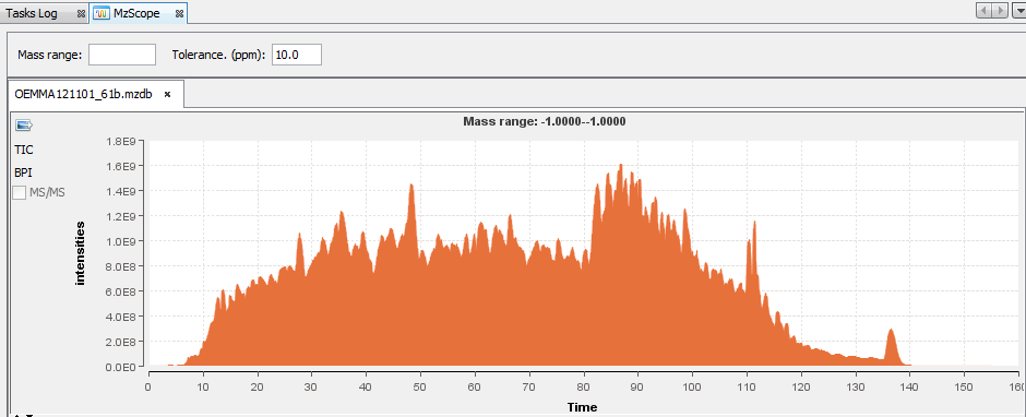
When the user chooses to “View” an mzDB file, the MzScope window is opened.
By default, the TIC chromatogram is displayed. You can click on “BPI” to see the best peak intensity graph.
By clicking in the graph, you can see below the scan at the selected time.
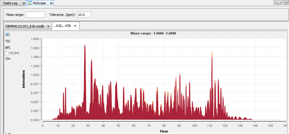
You can choose to display 2 or more chromatograms on the same graph, by selecting 2 files and clicking on “View”
You can extract a chromatogram at a given mass by entering the specified value in the panel above.
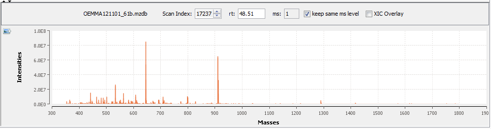
You can navigate through the scans
- by increasing or decreasing the scan Ids
- by entering a retention time
- by clicking the keys arrows on the keyboard (Ctrl+Arrows to keep the same ms level)
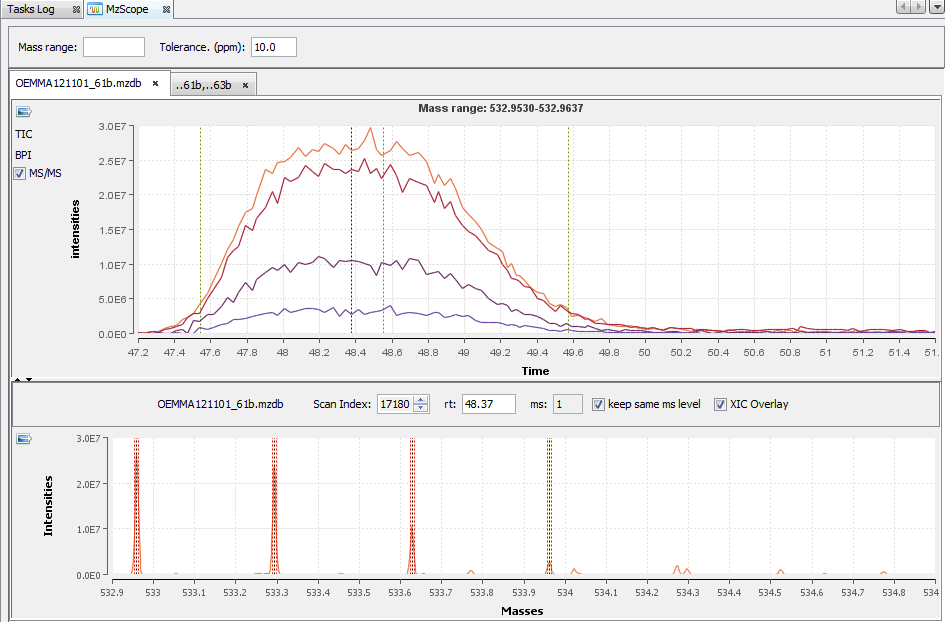
By double clicking on the scan, the corresponding chromatogram is displayed above (The Alt key or the check box “XIC overlay” allows you to overlay the chromatograms in the same graph).
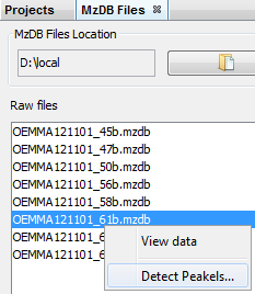
By selecting a file, you can click on “Detect Peakels” in the popup menu.
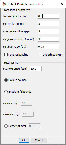
A dialog allows you to choose the parameters of the peakels detection: the tolerance and eventually a range of m/z, or a m/z value:
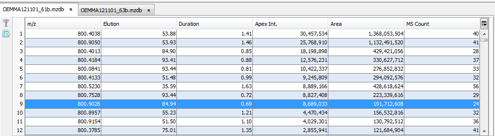
The results are displayed in a table:
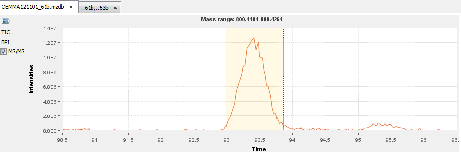
You can double-click (or through the popup menu) on a row to display the peakel in the corresponding raw file:
There are many ways to do an export:
- Export a Table using the export button (supported formats: {xlsx, xls, csv})
- Export data using Copy/Paste from the selected rows of a Table to an application like Excel.
- Export all data corresponding to an Identification Summary, XIC or Spectral Count
- Export an image of a view
- Export Identification Summary data into MzIdentML format ( for ProteomeXchange) .
- Export Identification Summary spectra list.
To export a table, click on the Export Button at the left top of a table.
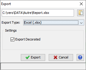
An Export Dialog is opened, you can select the file path for the export and the format of the export (supported formats: {xlsx, xls, csv}).
In case that the selected format is either .xls or .xlsx, the user has now the ability to maintain in his exported excel document any rich text format elements (color, font weight etc.) apparent on the original table in Proline Studio. Choice is done using the checkbox shown on the following screenshot.
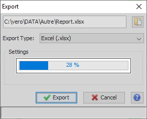
To perform the export, click on the Export Button. The task can take a few seconds if the table has a lot of rows and so a progress bar is displayed.
To copy/Paste a Table:
- Select rows you want to copy
- Press Ctrl and C keys at the same time. The column titles are also copied
- Open your spreadsheet editor and press Ctrl and V keys at the same time to paste the copied rows. If paste is done in a text editor, the column separator used is the tabulations.
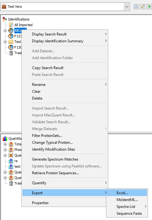
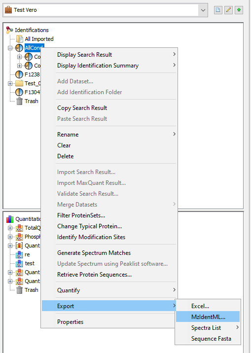
To Export all data of a dataset (Identification Summary, XIC or Spectral Count), right-click on the dataset to open the contextual menu and select the “Export” menu and then “Excel...” sub-menu.
You can also export multiple dataset simultaneously, if they have the same type (Identification Summary or XIC or Spectral Count).
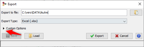
An Export Dialog is opened, you can select the file path and the type of the export : Excel (.xlsx) or Tabulation separated values (.tsv).
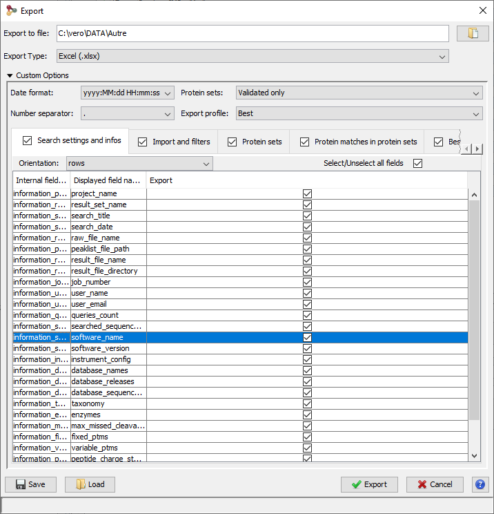
You can export with the default parameters or perform a custom export. To enable custom export, click on the tick box located on the right of the dialog:
Custom export allows a number of parameters in addition to the file format to be chosen.
Description of the exported file is available here.
Note: The parameters could be saved and loaded in further export using the Save / Load buttons of the export dialog.
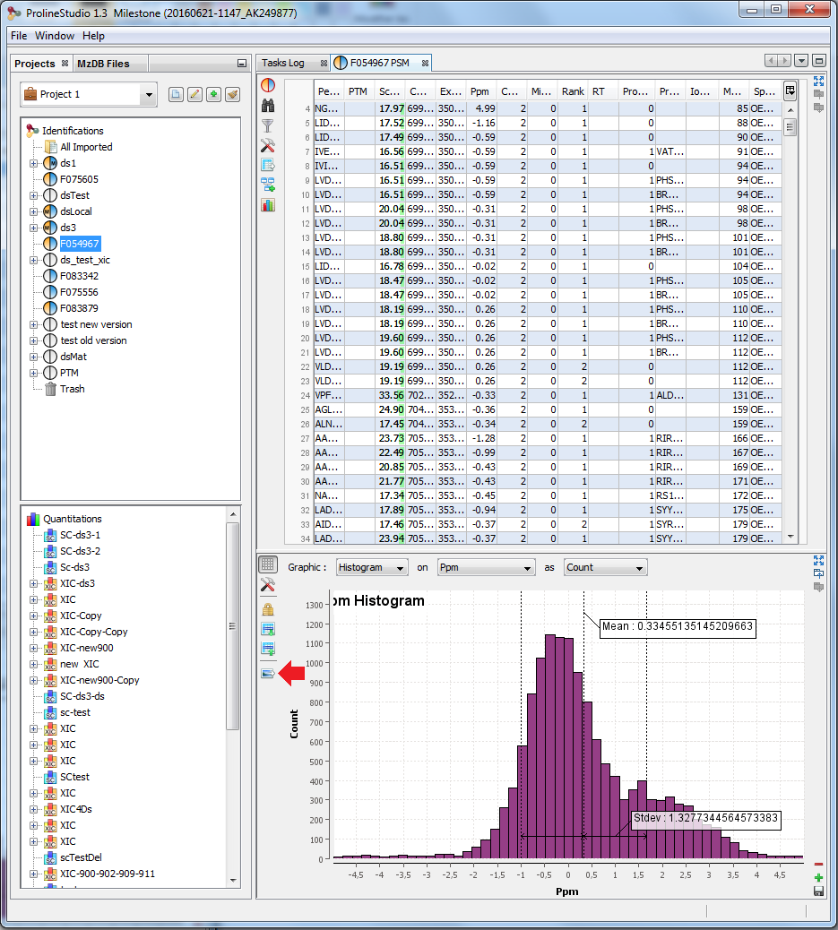
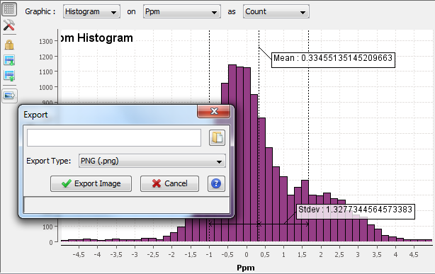
Any graphics in proline can be exported. Click on the Export Image Button at the left top of the image.
An Export Dialog is opened where you can select the file path and the export type. Available formats are PNG or SVG formats. SVG format produces a vector image that can be edited and resized afterwards.
Actually it is possible to export Identification Summary into MzIdentML, Pride isn’t supported any more.
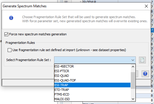
Note: Before exporting data all spectrum matches should have been generated. To do so, right click on the dataset and select “Generate Spectrum Matches”.
Right click on the dataset you want to export and select the “Export” menu and then “MzIdentML...” sub-menu
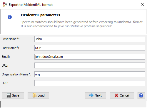
A dialog is opened where user information may be specified (name, organization …)
The file name and path should be specified in the next step. A progress bar is shown until the file is generated. The generated file contains identification and validation data issues from the dataset. All meta information including instrument configuration as well as search engine parameters are also extracted from dataset associated data.
To export valid PSM Spectra from an Identification Summary or from a XIC Dataset. The exported tsv file is compatible with Peakview.
Note: all Spectrum Matches must be generated first.
When importing a Search Result in Proline, users can view PSM with their associated Spectrum but by default no annotation is defined. Users need to generate (and save) this information explicitly.
In both cases, the following dialog will be opened. User can
Once executed, the dataset views need to be loaded again to effectively view the spectrum matches.
See description of Validation Algorithm.
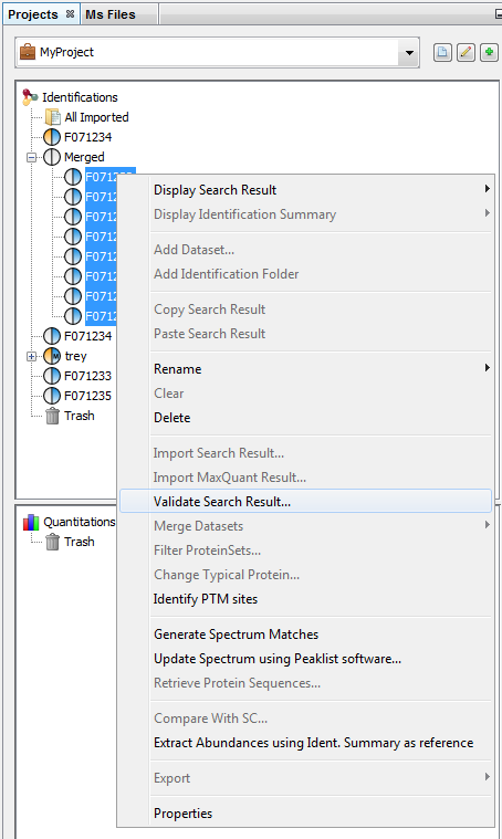
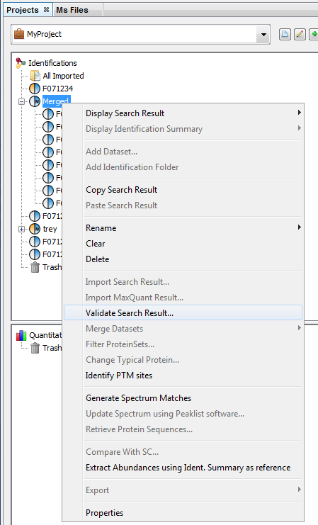
It is possible to validate identification Search Result or merged ones. In the latest case, the filters and validation threshold can be propagated to child Search Results.
To validate a Search Result:
- Select one or multiple Search Results to validate
- Right Click to display the popup
- Click on “Validate…” menu
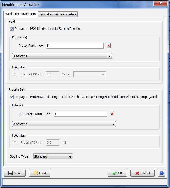
In the Validation Dialog, fill the different Parameters (see Validation description):
- you can add multiple PSM Prefilter Parameters ( Rank, Length, Score, e-Value, Identity p-Value, Homology p-Value) by selecting them in the combobox.
- you can ensure a FDR on PSMs which will be reached according to the variable selected ( Score, e-Value, Identity p-Value, Homology p-Value,… )
- you can add a Protein Set Prefilter on Specific Peptides count, peptides or peptides sequence count or on Protein Sets score.
- you can ensure a FDR on protein Sets.
Note: FDR can be used only for Search Results with Decoy Data.
If you run validation on a merged Search Result, you can choose to propagate it to child Search Result. Specified prefilters will be used as defined. For the FDR Filter, it is the threshold found by the validation algorithm which will be used for childs, as a prefilter.
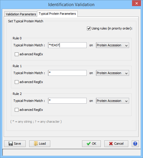
In the second tab, you can define rules for choosing the Typical Protein of a Protein Set by using a match string with wildcards ( * or ? ) on Protein Accession or Protein Description. (see Change Typical Protein of Protein Sets).
Note: All validation parameters can be saved and loaded using appropriated buttons.
Validating a Search Result can take some time. While it is not finished, the Search Results are shown greyed with an hourglass over them. The tasks are displayed as running in the “Tasks Log Dialog”.
When the validation is finished, the icon becomes orange and blue. Orange part corresponds to the Identification Summary. Blue is for the Search Result part.
See description of Protein Sets Filtering.
The protein sets windows are not updated after filtering Protein Set. You should close and reopen the window
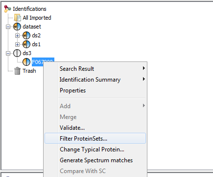
To filter Protein sets of Identification Summaries:
- Select one or multiple Identification Summaries to filter
- Right Click to display the popup
- Click on “Filter ProteinSets…” menu
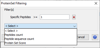
you can add multiple filters (Specific Peptides, Peptide count, Peptide sequence count, Protein Set Score) by selecting them in the combobox.
Once the filtering is done, you will have to open a new protein sets window in order to see modification.
The protein sets windows are not updated after changing Typical Protein. You should close and reopen the window
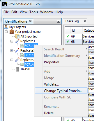
To change the Typical Protein of the Protein Sets of an Identification Summary:
- Select one or multiple Identification Summaries
- Right Click to display the popup
- Click on “Change Typical Protein…” menu
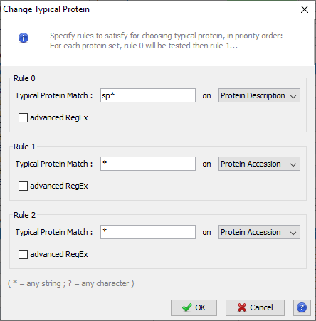
You can set the choice for the Typical Protein of Protein Sets by using a match string with wildcards (* or ?) on Protein Accession or Protein Description.
For Advanced users, a fully regular expression could be specified. In this case, check the corresponding option.
Three rules could be specified. They are applied in priority order, i.e. if no protein of a protein set satisfies the first rule, the second one is tested and so on.
The modification of Typical Proteins can take some time. During the processing, Identification Summaries are displayed grayed with an hourglass and the tasks are displayed in the Tasks Log Window
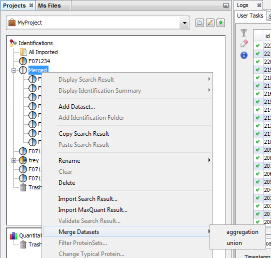
Merge can be done on Search Results or on Identification Summaries. You have also to specify which merge mode is to be used (aggregation or union). See description for combining Search Results or Identification Summaries.
To merge a dataset with multiple Search Results:
- Select the parent dataset
- Right Click to display the popup
- Click on “Merge” menu
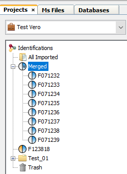
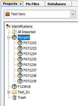
When the merge is finished, the dataset is displayed with an U or A in the blue part of the icon, indicating that the merge has been done using Union or Aggregation at a Search Result level.
If you merge a dataset containing Identification Summaries. The merge is done on an Identification Summary level. Therefore the dataset is displayed with an U or A in the orange part of the icon.
The purpose of the Data Analyzer is to easily do calculations/comparisons on data.
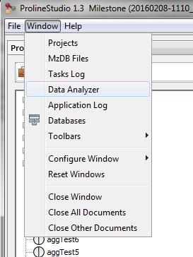
To open the data analyzer, you have two possibilities:
- you can use the dedicated button that you can find in the toolbar of all views. If you use this button, the corresponding data is directly sent to the data analyzer.
- you can use the menu “Window > Data Analyzer”
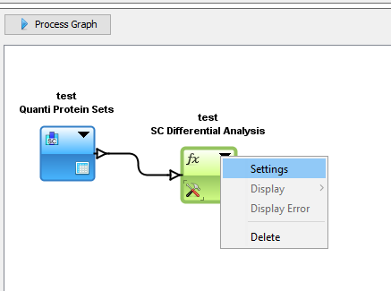
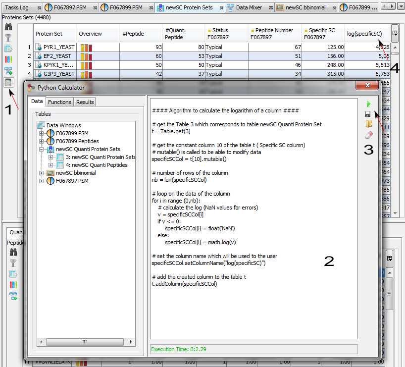
In the Data Analyzer view, you can access all data views, to some functions and graphics. In the following example, we create a graph by adding by Drag & Drop the Spectral Count Data and the corresponding differential analysis function (beta-binomial BBinomial). Then we link them together.
You have to specify the parameters of the Function: right click on the function and select the “settings” menu
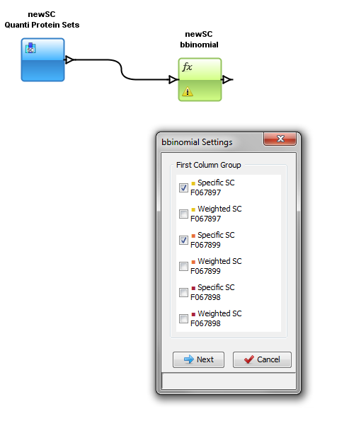
In the settings menu, select the two groups of columns on which you want to perform the BBinomial function. When the parameters are set, the calculation is started immediately and an hourglass icon is shown.
When the calculation is finished: the hourglass icon becomes a green tick, and the user can right click and select the “Display” menu to see the result (or click on the “table" icon).
This function is used by ProStar Macro to compute the FDR.
More information: http://bioconductor.org/packages/release/bioc/vignettes/Prostar/inst/doc/Prostar_UserManual.pdf
Calibration Plot for Proteomics is described here: https://cran.r-project.org/web/packages/cp4p/index.html
beta binomial function, useful for Spectral Count Quantitations
This function is used by ProStar Macro. Two tests are available: Welch t-test and Limma t-test.
More information: http://bioconductor.org/packages/release/bioc/vignettes/Prostar/inst/doc/Prostar_UserManual.pdf
This function is used by ProStar Macro to remove rows with too many missing quantitative values.
The available missing values algorithm are:
This function is used by ProStar Macro to impute missing values.
More information: http://bioconductor.org/packages/release/bioc/vignettes/Prostar/inst/doc/Prostar_UserManual.pdf
This function is used by ProStar Macro to normalize quantitative values.
More information on algorithms: http://bioconductor.org/packages/release/bioc/vignettes/Prostar/inst/doc/Prostar_UserManual.pdf
Join data from two tables according to the selected key.
Perform a difference between two joined table data according to a selected key. When a key value is not found in one of the data source tables, the line is displayed as empty. For numerical values a difference is done and for string values, the '<>' symbol is displayed when values are different.
Columns filter, let the user remove unnecessary columns in a matrix. A combobox, with prefix and suffix of the columns allows to select multiple similar columns to filter them rapidly.
Rows filter function lets the user filter some rows of a matrix according to settings on columns.
Create a column by calculating the Log (2 or 10) of an existing column.
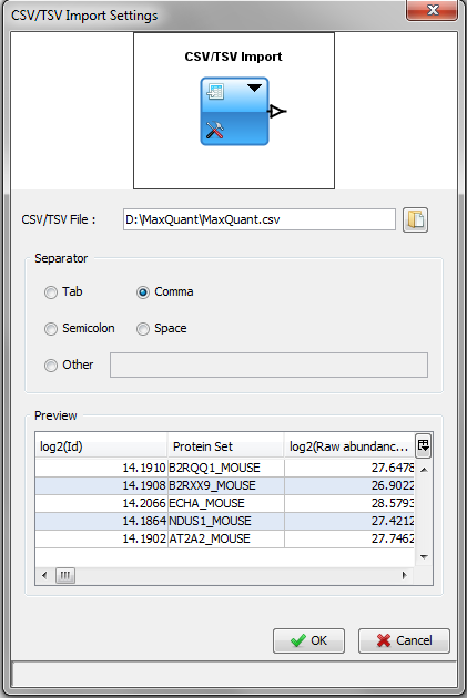
This module lets you import data from a CSV or TSV file. Then you can do calculations and display these data directly in Proline Studio.
The separator is automatically selected according to the csv file. But you can modify it.
The preview zone displays the first lines of the file as it will be loaded.
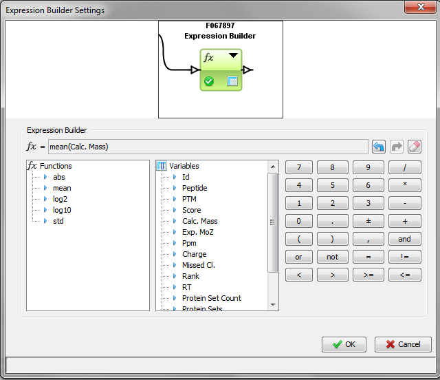
The expression builder lets you create an expression with built-in functions or comparators and variables (columns from the linked matrix). In the example, we calculate the mean of a column in the matrix.
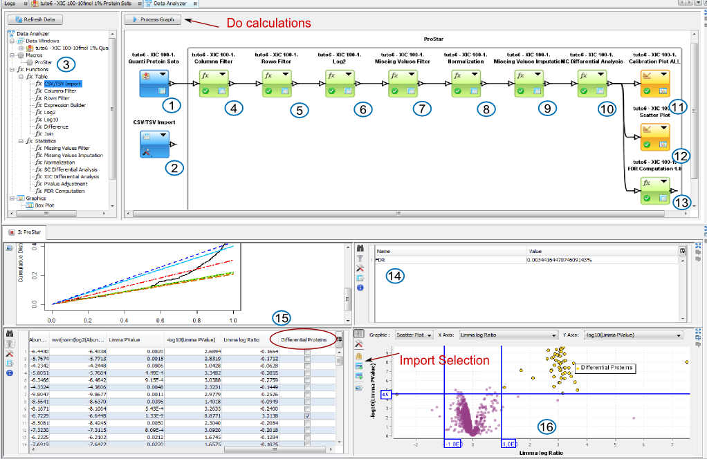
1 or 2: Add XIC Data to Data Analyzer from the Protein Set View or by importing data from a csv file.
3: Add Prostar Macro by a drag and drop and link XIC Data to the Macro. And do the calculation by clicking on the button Process Graph.
During the process, the Data Analyzer will ask you settings for each function.
4: Filter unnecessary columns from your data if. Settings can be validated with no parameters if you don't need it.
5: Filter is needed only if you want to remove contaminants. Settings can be validated with no parameters if you don't need it.
6: Log is needed to log abundances (Data from Proline). For Data coming from MaxQuant, data is already logged.
7 to 13: follow the settings asked ( you can find some help in Prostar documentation, or information in corresponding functions.)
During the process, results will be automatically displayed:
14: FDR Result
15: Calibration Plots
16: Result Table with differential Proteins Table and the corresponding scatter plot. You can select differential proteins in the table, to import them in the scatter plot and create a colored group with them.
If you want to look at other results, right click on a function and select “Display in New Window”
Prostar User Manual:
http://bioconductor.org/packages/release/bioc/vignettes/Prostar/inst/doc/Prostar_UserManual.pdf
Prostar Tutorial :
http://bioconductor.org/packages/release/bioc/vignettes/Prostar/inst/doc/Prostar_Tutorial.pdf
Calculator lets you write python scripts to manipulate freely viewed data.
1) To open the calculator, click on the calculator icon (not available on all views for the moment)
On the left part of the calculator, you can access all viewed data, double click to add a table or a column to the script.
2) Write your python script on the text area
3) Execute it by clicking on the green Arrow.
4) When the script has been executed, the results of the calculations (variables, new columns) are available in the “Results” tab. Double click on a new column to add it to the table. Or like in the example, directly add the column to the table programmatically.
#### Algorithm to calculate the logarithm of a column ####
# get the Table 3 which corresponds to table newSC Quanti Protein Set
t = Table.get(3)
# get the constant column 10 of the table t ( Specific SC column)
# mutable() is called to be able to modify data
specificSCCol = t[10].mutable()
# number of rows of the column
nb = len(specificSCCol)
# loop on the data of the column
for i in range (0,nb):
# calculate the log (NaN values for errors)
v = specificSCCol[i]
if v <= 0:
specificSCCol[i] = float('NaN')
else:
specificSCCol[i] = math.log(v)
# set the column name which will be used to the user
specificSCCol.setColumnName("log(specificSC)")
# add the created column to the table t
t.addColumn(specificSCCol)
#### Algorithm to perform a difference and a mean between two columns ####
t = Table.get(9)
colAbundance1 = t[3]
colAbundance2 = t[5]
# difference between two columns
colDiff = colAbundance1-colAbundance2
# set the name of the column
colDiff.setColumnName("diff")
# mean between two columns
colMean = (colAbundance1+colAbundance2)/2
# set the name of the column
colMean.setColumnName("mean")
# add columns to the table
t.addColumn(colDiff)
t.addColumn(colMean)
#### Algorithm to perform a pvalue and a ttd on abundances column of a XIC quantitation ####
t = Table.get(1)
pvalueCol = Stats.pvalue( (t[2], t[3]), (t[4],t[5]) )
ttdCol = Stats.ttd( (t[2], t[3]), (t[4],t[5]) )
pvalueCol.setColumnName("pvalue")
ttdCol.setColumnName("ttd")
t.addColumn(pvalueCol)
t.addColumn(ttdCol)
When importing a search result, the software used for the peaklist creation has to be specified. This parameter is mandatory for the XIC quantitation as it is used to find scan number or RT in the spectrum title. Indeed, this information is then used to extract abundances in the raw files.
If an invalid software has been specified when importing, it is possible to change the peaklist software afterwards. This option is only valid for Identification DataSets.
Right click on the identification DataSet, and select “Update Spectrum using Peaklist software”
The following dialog will be displayed allowing the user to select the peaklist software to use.
See description of Compare Identification Summaries with Spectral Count.
To obtain a spectral count, right click on a Dataset with merged Identification Summaries and select the “Quantify → Spectral Counting” menu in the popup. This Dataset is used as the reference Dataset and Protein Set list as well as specifics peptides are defined there.
In the Spectral Count window, fill the name and description of your Spectral Count and press Next.
Then select the Identification Summaries on which you want to perform the Spectral Count and press Next.
Finally select the DataSet where shared peptides spectral count weight should be calculated and press OK.
A Spectral Count is created and added to the Quantitations Panel.
You can then display a Spectral Count, see Display a Spectral Count
For description on LC-MS Quantitation you can first read the principles in this page: Quantitation: principles
You can create a new XIC design by clicking on the “Quantify → Label Free” menu from Quantitation or from a dataset in the Identification tree. In this case, the selected dataset will be used as reference for the quantitation (from where the list of peptides and protein is extracted).
When you start the creation of a new XIC Design, the following dialog is opened:
In the left Area, you can create your design :
From the right Area, you can drag and drop desired identifications to the left Area. If you drop in the XIC or in a Group node, Group and Sample nodes will be automatically added. But you can drop directly in a Sample node.
Note : it is recommended that the XIC node is renamed.
When your design is ready, click on Next Button.
The following panel is displayed:
In order to be able to perform any XiC design, all participating Sample Analysis must be associated with a corresponding raw file. The association is done at the second step of the XIC design by :
When all participating Sample Analysis are associated with a raw file, click on Next Button.
Now you must select the parameters. See Label-free LC-MS quantitation configuration to have more details about the different parameters.
The XIC parameters are not all displayed. You can display a complete set of parameters by clicking on the “Advances Parameters”.
Note: all the parameters are already set with default values.
You can copy a XIC design by selecting the “Clone & Extract Abundances” option from an existing quantitation result. The new XIC is generated using an existing Experimental Design and parameters setting.
Newly generated XIC designs are immediately added to the Quantitation Tree. Through the latter one, and via a popup menu, the end user has the capacity either to view a design’s properties as seen to the following screenshot, or to apply a series of actions on it, including among others:
It is possible to aggregate data from different XIC designs.
First you must select two or more XIC Designs in the Quantitation tree and do a mouse right click to obtain a popup and then select the menu “Aggregate Quantitations”.
The following dialog is opened:
This dialog is divided in three areas:
You can completely modify the inferred aggregated experimental design. You can use drag & drop to modify the order of the items and the right mouse popup to create, delete or rename items.
You can modify the quantitation channels mapping by drag and drop from the right area to the center area. You can also remove or reorder the mapping thanks to the right mouse popup or thanks to the floating panel.
When you select a Channel, you can click on the help button to check what the aggregation will exactly do.
Right click on the selected XIC node in the Quantitation tree, and select “Compute Post Processing on Abundances…”
In the dialog, you can:
- specify peptides to consider for quantitation
- configure parameters used for peptides quantitation
- configure parameters used for proteins quantitation
For more details, see Post-processing of LC-MS quantitative results
You can see the results by displaying the XIC (Display a XIC) or export them Export Data
Since version 1.4 Proline Studio includes a general settings dialog which can be accessed from the top menu bar clicking on “General Settings” as shown in the screenshot below.
The latter one consists of a constantly but slowly growing number of user preferences regarding various aspects of the utilization of Proline Studio. Based on their context, for the time being, preferences are organized into the following four tabs:
JMS Settings tab contains parameters that concern the exchange of messages between your local machine and the JMS Server. It should be made clear that compared to other preferences, preferences that are included in this tab should be treated with caution. Mistreating a communication preference can lead either to communication/connection problems or to users’ confusion to whether they are connected to the correct server version.
Parameter can be seen as a name which represents a server address. The parameter’s existence is justified by the fact that multiple server versions might run on the same server machine imposing the need to be able to canalize Studio’s messages appropriately.
Table parameters’ tab encapsulates a short list of preferences regarding all tables generated throughout Proline Studio. More specifically those preferences control the arrangement of the participating columns as well as their respective width.
This field dictates the spatial arrangement of table columns. Three arrangements are possible:
When “Automatic Columns Size” is used, all columns are width-wise readjusted in a way that they all fit to their container. Given that it is a “fit-to-screen” approach, it lacks scrollbars and does not guarantee the readability of the presented date, especially when the number of columns is high.
On the other hand a simpler approach that guarantees readability is to select “Fixed Column Size”. In this case all table columns have a fixed width, explicitly dictated by the user using the parameter “Column Width”.
The less clear option is “Smart Column Size” which serves as a trade off between the aforementioned ones. It tackles with the cases that either we have too many columns to visualize using the “Automatic” approach or too few and the selected default and globally applied width imposes unneeded scrollbars ending in hiding some columns at the same time. In this context, “Smart Column Size” can be seen as a simple rule based on the ratio between the mean column width needed in case of “Automatic Column Size” for a specific table and the globally selected width. For the sake of simplicity we have set a threshold of 0.7 or 70% which on its turn determines which one of the two first modes will be used given a table. If the ratio is smaller than 0.7 then the table in question will be presented in “Fixed Column Size” mode. On contraire if ratio is equal or greater than 0.7, then we consider that using “Automatic Column Size” mode is more appropriate as it balances between a possible slightly smaller than desired width and the possibility of hiding a column using scrollbars.
The second preference is more or less self explanatory and corresponds to the globally desired columns’ width when fixed rune is applied, either directly or as a result of the smart mode.
In this tab we can find a diverse set of preferences regarding various tasks encountered in Proline Studio. For the time being those preferences are:
Unlike the last three, Hide Getting Started Dialog is pretty much self explanatory. The second preference on the other hand, “Default Search Name Source” affects the way identification datasets are named on importation. For this preference we have three possible options:
This parameter affects the .xls and .xlsx files that are produced in the process of export (client side). It could be easily described as a preservation of any existing Rich Text Feature in a table. (Colors, Font Weight etc.)
Corresponds to the default raw2mzDB converter. While it is left at the discretion of the user, which version to choose, it must be noted that different versions do tend to work better with specific type raw files. Said that, it is also important to understand that in order for a conversion to be successful within Proline Studio, all system requirements set by the specific raw2mzDB version must be met.
For description on sites and clusters you can first read the principles in this page: Identifying Modification sites and clusters
To identify Modification sites and create Modification clusters, right click on the Identification Summary and select Identify Modification sites.
A dialog is displayed where you can choose Modification of interest and configure the clustering method (see Identifying Modification sites and clusters for more details).
Some administration views and operations are accessible through Proline Studio File > Admin menu. Some edit functions are only permitted to advanced users, who at the same time hold the status of Admin..
The “User Accounts” tab, list all registered users with the group they belong to. Admin users can add new users or modify existing one. Modifications consist in changing user groups or password.
User account modification dialog
Peaklist Softwares tab permits users to view the list of all available Peaklist Software. A detailed view could be displayed when selecting the “View Peaklist Software” button.
In both windows, It is possible to test a spectrum title to verify which data are extracted for a given Peaklist Software.
Admin users also have the possibility to add new Peaklist Software definition (name, version and extraction rules using regular expression) or to modify existing definitions by changing the name or version. Rules are not modifiable since some already parsed data may not be consistent with the new definition. New rules definition may be done by creation of a new peaklist software.
A faire
a Faire